Multiple Regression

Data-Based Economics, ESCP, 2024-2025

The problem

Remember dataset from last time

	type	income	education	prestige
accountant	prof	62	86	82
pilot	prof	72	76	83
architect	prof	75	92	90
author	prof	55	90	76
chemist	prof	64	86	90

• Last week we “ran” a linear regression: $y=\alpha +\beta x$. Result: $$\text{income}=xx+0.72\text{education}$$
• Should we have looked at “prestige” instead ? $$\text{income}=xx+0.83\text{prestige}$$
• Which one is better?

---

Prestige or Education

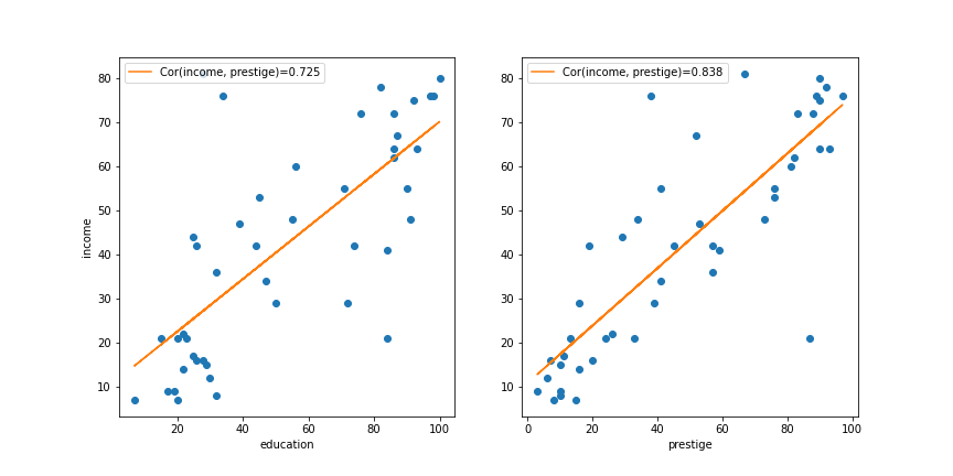
• if the goal is to predict: the one with higher explained variance
  • prestige has higher $R^2$ (${0.83}^2$)
• unless we are interested in the effect of education

---

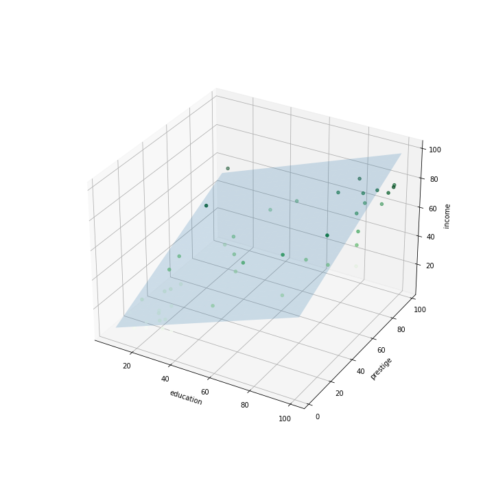
Multiple regression

• What about using both?
  • 2 variables model: $$\text{income}=\alpha +{\beta }_1\text{education}+{\beta }_2\text{prestige}$$
  • will probably improve prediction power (explained variance)
  • ${\beta }_1$ might not be meaningful on its own anymore (education and prestige are correlated)

---

Fitting a model

Now we are trying to fit a plane to a cloud of points.

---

Minimization Criterium

• Take all observations: $({\text{income}}_n,{\text{education}}_n,{\text{prestige}}_n{)}_{n\in [0,N]}$
• Objective: sum of squares $$L(\alpha ,{\beta }_1,{\beta }_2)=\sum _i{\left(\underset{e_n=\text{prediction error}}{\underbrace{\alpha +{\beta }_1{\text{education}}_n+{\beta }_2{\text{prestige}}_n-{\text{income}}_n}}\right)}^2$$
• Minimize loss function in $\alpha$, ${\beta }_1$, ${\beta }_2$
• Again, we can perform numerical optimization (machine learning approach)
  • … but there is an explicit formula

---

Ordinary Least Square

$$Y=\left[\begin{array}{c}{\text{income}}_1\\ \\ ⋮\\ \\ {\text{income}}_N\end{array}\right]$$ $$X=\left[\begin{array}{ccc}1& {\text{education}}_1& {\text{prestige}}_1\\ \\ ⋮& ⋮& ⋮\\ \\ 1& {\text{education}}_N& {\text{prestige}}_N\end{array}\right]$$

• Matrix Version (look for $B=(\alpha ,{\beta }_1,{\beta }_2)$): $$Y=XB+E$$
• Note that constant can be interpreted as a “variable”
• Loss function $$L(A,B)=(Y-XB{)}^{\prime }(Y-XB)$$
• Result of minimization $\underset{(A,B)}{min}L(A,B)$ : $$\left[\begin{array}{ccc}\alpha & {\beta }_1& {\beta }_2\end{array}\right]=(X^{\prime }X{)}^{-1}{X}^{\prime }Y$$

Solution

• Result: $$\text{income}=10.43+0.03\times \text{education}+0.62\times \text{prestige}$$
• Questions:
  • is it a better regression than the other?
  • is the coefficient in front of education significant?
  • how do we interpret it?
  • can we build confidence intervals?

Explained Variance

Explained Variance

As in the 1d case we can compare: - the variability of the model predictions ($MSS$) - the variance of the data ($TSS$, T for total)

Coefficient of determination (same formula):

$$R^2=\frac{MSS}{TSS}$$

Or:

$$R^2=1-\frac{RSS}{SST}$$

where $RSS$ is the non explained variance

Adjusted R squared

Fact:

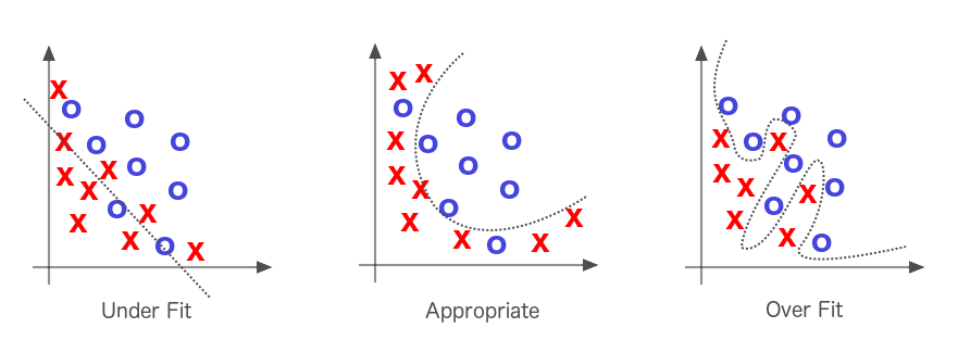
• adding more regressors always improve $R^2$
• why not throw everything in? (kitchen sink regressions)
• two many regressors: overfitting the data

Penalise additional regressors: adjusted R^2

$$R_{adj}^2=1-(1-R^2)\frac{N-1}{N-p-1}$$

Where:

• $N$: number of observations
• $p$ number of variables

In our example:

Regression	$R^2$	$R_{adj}^2$
education	0.525	0.514
prestige	0.702	0.695
education + prestige	0.7022	0.688

Interpretation and variable change

Making a regression with statsmodels

import statsmodels

We use a special API inspired by R:

import statsmodels.formula.api as smf

Performing a regression

• Running a regression with statsmodels

model = smf.ols('income ~ education',  df)  # model
res = model.fit()  # perform the regression
res.describe()

• ‘income ~ education’ is the model formula

                            OLS Regression Results                            
==============================================================================
Dep. Variable:                 income   R-squared:                       0.525
Model:                            OLS   Adj. R-squared:                  0.514
Method:                 Least Squares   F-statistic:                     47.51
Date:                Tue, 02 Feb 2021   Prob (F-statistic):           1.84e-08
Time:                        05:21:25   Log-Likelihood:                -190.42
No. Observations:                  45   AIC:                             384.8
Df Residuals:                      43   BIC:                             388.5
Df Model:                           1                                         
Covariance Type:            nonrobust                                         
==============================================================================
                 coef    std err          t      P>|t|      [0.025      0.975]
==============================================================================
Intercept     10.6035      5.198      2.040      0.048       0.120      21.087
education      0.5949      0.086      6.893      0.000       0.421       0.769
==============================================================================
Omnibus:                        9.841   Durbin-Watson:                   1.736
Prob(Omnibus):                  0.007   Jarque-Bera (JB):               10.609
Skew:                           0.776   Prob(JB):                      0.00497
Kurtosis:                       4.802   Cond. No.                         123.
==============================================================================

Formula mini-language

• With statsmodels formulas, can be supplied with R-style syntax
• Examples:

Formula	Model
income ~ education	${\text{income}}_i=\alpha +\beta {\text{education}}_i$
income ~ prestige	${\text{income}}_i=\alpha +\beta {\text{prestige}}_i$
income ~ prestige - 1	${\text{income}}_i=\beta {\text{prestige}}_i$ (no intercept)
income ~ education + prestige	${\text{income}}_i=\alpha +{\beta }_1{\text{education}}_i+{\beta }_2{\text{prestige}}_i$

Formula mini-language

• One can use formulas to apply transformations to variables

Formula	Model
log(P) ~ log(M) + log(Y)	$\log (P_i)=\alpha +{\alpha }_1\log (M_i)+{\alpha }_2\log (Y_i)$ (log-log)
log(Y) ~ i	$\log (P_i)=\alpha +i_i$ (semi-logs)

• This is useful if the true relationship is nonlinear
• Also useful, to interpret the coefficients

Coefficients interpetation

Example:

• (police_spending and prevention_policies in million dollars) $$\text{text{number\_or\_crimes} = 0.005\% - 0.001 text{pol\_spend} - 0.005 text{prev\_pol} + 0.002 text{population density}}$$

• reads: when holding other variables constant a 0.1 million increase in police spending reduces crime rate by 0.001%

Iinterpretation?

• problematic because variables have different units
• we can say that prevention policies are more efficient than police spending ceteris paribus

Take logs: $$\text{log(text{number\_or\_crimes}) = 0.005\% - 0.15 log(text{pol\_spend}) - 0.4 log(text{prev\_pol}) + 0.2 log(text{population density})}$$

• now we have an estimate of elasticities
• a $1\mathrm{\%}$ increase in police spending leads to a $0.15\mathrm{\%}$ decrease in the number of crimes

Statistical Inference

Hypotheses

• Recall what we do:
  • we have the data $X,Y$
  • we choose a model: $$Y=\alpha +X\beta$$
  • from the data we compute estimates: $$\hat{\beta }=(X^{\prime }X{)}^{-1}{X}^{\prime }Y$$ $$\hat{\alpha }=Y-X\beta$$
  • estimates are a precise function of data
    • exact formula not important here

We need some hypotheses on the data generation process:

• $Y=X\beta +ϵ$
• $\mathbb{E}\left[ϵ\right]=0$
• $ϵ$ multivariate normal with covariance matrix ${\sigma }^2{I}_n$
  • $\mathrm{\forall }i,\sigma ({ϵ}_i)=\sigma$
  • $\mathrm{\forall }i,j,cov({ϵ}_i,{ϵ}_j)=0$

Under these hypotheses:

• $\hat{\beta }$ is an unbiased estimate of true parameter $\beta$
  • i.e. $\mathbb{E}[\hat{\beta }]=\beta$
• one can prove $Var(\hat{\beta })={\sigma }^2{I}_n$
• $\sigma$ can be estimated by $\hat{\sigma }=S\frac{\sum _i(y_i-{pred}_i{)}^2}{N-p}$
  • $N-p$: degrees of freedoms
• one can estimate: $\sigma (\widehat{{\beta }_k})$
  • it is the $i$-th diagonal element of ${\hat{\sigma }}^2{X}^{\prime }X$

Is the regression significant?

• Approach is very similar to the one-dimensional case

Fisher Criterium (F-test)

• $H0$: all coeficients are 0
  • i.e. true model is $y=\alpha +ϵ$
• $H1$: some coefficients are not 0

Statistics: $$F=\frac{MSR}{MSE}$$ (same as 1d)

• $MSR$: mean-squared error of constant model
• $MSE$: mean-squared error of full model

Under:

• the model assumptions about the data generation process
• the H0 hypothesis

… the distribution of $F$ is known

It is remarkable that it doesn’t depend on $\sigma$ !

One can produce a p-value.

• probability to obtain this statistics given hypothesis H0
• if very low, H0 is rejected

Is each coefficient significant ?

Student Test

Given a coefficient ${\beta }_k$:

• $H0$: true coefficient is 0
• $H1$: true coefficient is not zero

Statistics (student-t): $$t=\frac{\widehat{{\beta }_k}}{\hat{\sigma }(\widehat{{\beta }_k})}$$

• where $\hat{\sigma }({\beta }_k)$ is $i$-th diagonal element of ${\hat{\sigma }}^2{X}^{\prime }X$
• it compares the estimated value of a coefficient to its estimated standard deviation

Under the inference hypotheses, distribution of $t$ is known.

• it is a student distribution

Procedure:

• Compute $t$. Check acceptance threshold $t\ast$ at probability $\alpha$ (ex 5%)
• Coefficient is significant with probability $1-\alpha$ if $t>t\ast$

Or just look at the p-value:

• probability that $t$ would be as high as it is, assuming $H0$

Confidence intervals

Same as in the 1d case.

• Take estimate ${\beta }_i$ with an estimate of its standard deviation $\hat{\sigma }({\beta }_i)$
• Compute student $t^{\star }$ at $\alpha$ confidence level (ex: $\alpha =5$) such that:
  • $P(|t|>t^{\star })<\alpha$

. . .

Produce confidence intervals at $\alpha$ confidence level:

• $[{\beta }_i-t^{\star }\hat{\sigma }({\beta }_i),{\beta }_i+t^{\star }\hat{\sigma }({\beta }_i)]$

Interpretation:

• for a given confidence interval at confidence level $\alpha$…
• the probability that our coefficient was obtained, if the true coefficient were outside of it, is smaller than $\alpha$

Other tests

• The tests seen so far rely on strong statistical assumptions (normality, homoscedasticity, etc..)
• Some tests can be used to test these assumptions:
  • Jarque-Bera: is the distribution of data truly normal
  • Durbin-Watson: are residuals autocorrelated (makes sense for time-series)
  • …
• In case assumptions are not met…
  • … still possible to do econometrics
  • … but beyond the scope of this course

Variable selection

Variable selection

• I’ve got plenty of data:
  • $y$: gdp
  • $x_1$: investment
  • $x_2$: inflation
  • $x_3$: education
  • $x_4$: unemployment
  • …

• Many possible regressions:
  • $y=\alpha +{\beta }_1{x}_1$
  • $y=\alpha +{\beta }_2{x}_2+{\beta }_3{x}_4$
  • …

. . .

• Which one do I choose ?
  • putting everything together is not an option (kitchen sink regression)

Not enough coefficients

Suppose you run a regression: $$y=\alpha +{\beta }_1{x}_1+ϵ$$ and are genuinely interested in coefficient ${\beta }_1$

. . .

But unknowingly to you, the actual model is $$y=\alpha +{\beta }_1{x}_1+{\beta }_2{x}_2+\eta$$

. . .

The residual $y-\alpha -{\beta }_1{x}_1$ is not white noise

• specification hypotheses are violated
• estimated $\widehat{{\beta }_1}$ will have a bias (omitted variable bias)
• to correct the bias we add $x_2$
  • even though we are not interested in $x_2$ by itself
  • we control for $x_2$

Example

• Suppose I want to check Okun’s law. I consider the following model: $$\text{text{gdp\_growth} = alpha + beta times text{unemployment}}$$
• I obtain: $$\text{text{gdp\_growth} = 0.01 - 0.1 times text{unemployment} + e\_i}$$
• Then I inspect visually the residuals: not normal at all!
• Conclusion: my regression is misspecified, $0.1$ is a biased (useless) estimate
• I need to control for additional variables. For instance: $$\text{text{gdp\_growth} = alpha + beta\_1 text{unemployment} + beta\_2 text{interest rate}}$$
• Until the residuals are actually white noise

Colinear regressors

• What happens if two regressors are (almost) colinear? $$y=\alpha +{\beta }_1{x}_1+{\beta }_2{x}_2$$ where $x_2=\kappa x_1$
• Intuitively: parameters are not unique
  • if $y=\alpha +{\beta }_1{x}_1$ is the right model…
  • then $y=\alpha +{\beta }_1\lambda x_1+{\beta }_2(1-\lambda )\frac{1}{\kappa }{x}_2$ is exactly as good…
• Mathematically: $(X^{\prime }X)$ is not invertible.
• When regressors are almost colinear, coefficients can have a lot of variability.
• Test:
  • correlation statistics
  • correlation plot

Choosing regressors

$$y=\alpha +{\beta }_1{x}_1+...{\beta }_n{x}_n$$

Which regressors to choose ?

Method 1 : remove coefficients with lowest t (less significant) to maximize adjusted R-squared

• remove regressors with lowest t
  • not the one you are interested in ;)
• regress again
• see if adjusted $R^2$ is decreasing
  • if so continue
  • otherwise cancel last step and stop

Method 2 : choose combination to maximize Akaike Information Criterium

• AIC: $p-log(L)$
• $L$ is likelihood
• computed by all good econometric softwares

Coming next

Intro to causality