Dataframes
Data-Based Economics
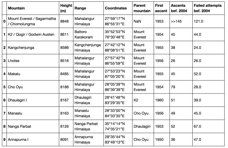
Tabular Data
DataFrame
- A DataFrame (aka a table) is a 2-D labeled data structure with columns
- each column has a specific type and a column name
- types: quantitative, qualitative (ordered, non-ordered, …)
- First column is special: the index
- first goal of an econometrician: constitute a good dataframe
- aka “cleaning the data”
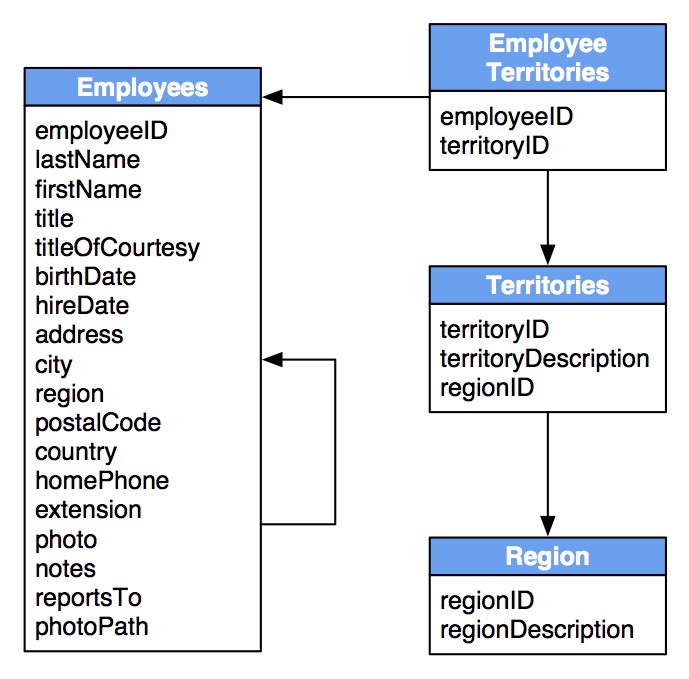
DataFrames are everywhere
- sometimes data comes from several linked dataframes
- relational database
- can still be seen conceptually as one dataframe…
- … through a join operation
- dataframes / relational databases are so ubiquitous a language has been developed for them
- SQL
- in the 80s…
- probably worth looking at if you have some “data” ambitions
- you will see the shadow of SQL everywhere - words like: join, merge, select, insert…
- plenty of resources to learn (example: sqbolt)
Pandas

pandas
- pandas = panel + datas
- a python library created by WesMcKinney
- very optimized
- essentially a dataframe object
- many options but if in doubt:
- minimally sufficient pandas is a small subset of pandas to do everything
- tons of online tutorials
creating a dataframe (1)
- Import pandas
- preferably with standard alias
pd
import pandas as pd - preferably with standard alias
- Import a dataframe
- each line a different entry in a dictionary
# from a dictionary
d = {
  "country": ["USA", "UK", "France"],
  "comics": [13, 10, 12]
}
pd.DataFrame(d)
| country | comics | |
|---|---|---|
| 0 | USA | 13 |
| 1 | UK | 10 |
| 2 | France | 12 |
creating a dataframe (2)
- there are many other ways to create a dataframe
- for instance using a numpy matrix (numpy is a linear algebra library)
# from a matrix
import numpy as np
M = np.array(
    [[18, 150],
     [21, 200],
     [29, 1500]]
)
df = pd.DataFrame( M, columns=["age", "travel"] )
df
| age | travel | |
|---|---|---|
| 0 | 18 | 150 |
| 1 | 21 | 200 |
| 2 | 29 | 1500 |
File Formats
Common file formats
- comma separated files:
csvfile- often distributed online
- can be exported easily from Excel or LibreOffice
- stata files: use
pd.read_dta() - excel files: use
pd.read_excel()orxlsreaderif unlucky- note that excel does not store a dataframe (each cell is potentially different)
- postprocessing is needed
Comma separated file
- one can actually a file from python
txt = """year,country,measure
2018,"france",950.0
2019,"france",960.0
2020,"france",1000.0
2018,"usa",2500.0
2019,"usa",2150.0
2020,"usa",2300.0
"""
open('dummy_file.csv','w').write(txt) # we write it to a file- and import it
df = pd.read_csv('dummy_file.csv') # what index should we use ?
df| year | country | measure | |
|---|---|---|---|
| 0 | 2018 | france | 950.0 |
| 1 | 2019 | france | 960.0 |
| 2 | 2020 | france | 1000.0 |
| 3 | 2018 | usa | 2500.0 |
| 4 | 2019 | usa | 2150.0 |
| 5 | 2020 | usa | 2300.0 |
“Annoying” Comma Separated File
- Sometimes, comma-separated files, are not quite comma-separated…
- inspect the file with a text editor to see what it contains
- the kind of separator, whether there are quotes…
txt = """year;country;measure
2018;"france";950.0
2019;"france";960.0
2020;"france";1000.0
2018;"usa";2500.0
2019;"usa";2150.0
2020;"usa";2300.0
"""
open('annoying_dummy_file.csv','w').write(txt) # we write it to a file
- inspect the file with a text editor to see what it contains
- add relevant options to
pd.read_csvand check result
pd.read_csv("annoying_dummy_file.csv", sep=";")| year | country | measure | |
|---|---|---|---|
| 0 | 2018 | france | 950.0 |
| 1 | 2019 | france | 960.0 |
| 2 | 2020 | france | 1000.0 |
| 3 | 2018 | usa | 2500.0 |
| 4 | 2019 | usa | 2150.0 |
| 5 | 2020 | usa | 2300.0 |
Exporting a DataFrame
pandas can export to many formats:
df.to_...to (standard) CSV
print( df.to_csv() ),year,country,measure
0,2018,france,950.0
1,2019,france,960.0
2,2020,france,1000.0
3,2018,usa,2500.0
4,2019,usa,2150.0
5,2020,usa,2300.0- or to stata
df.to_stata('dummy_example.dta')Data Sources
Types of Data Sources
- Where can we get data from ?
- check one of the databases lists kaggle, econ network
- Official websites
- often in csv form
- unpractical applications
- sometimes unavoidable
- open data trend: more unstructured data
- Data providers
- supply an API (i.e. easy to use function)
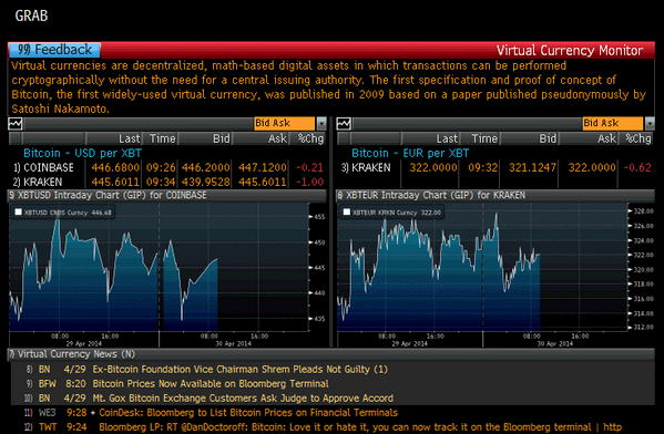
Data providers
- commercial ones:
- bloomberg, macrobond, factsets, quandl …
- free ones available as a python library
dbnomics: many official time-seriesqeds: databases used by quanteconvega-datasets: distributed with altair
import vega_datasets
df = vega_datasets.data('iris')
df| sepalLength | sepalWidth | petalLength | petalWidth | species | |
|---|---|---|---|---|---|
| 0 | 5.1 | 3.5 | 1.4 | 0.2 | setosa |
| 1 | 4.9 | 3.0 | 1.4 | 0.2 | setosa |
| 2 | 4.7 | 3.2 | 1.3 | 0.2 | setosa |
| 3 | 4.6 | 3.1 | 1.5 | 0.2 | setosa |
| 4 | 5.0 | 3.6 | 1.4 | 0.2 | setosa |
| … | … | … | … | … | … |
| 145 | 6.7 | 3.0 | 5.2 | 2.3 | virginica |
| 146 | 6.3 | 2.5 | 5.0 | 1.9 | virginica |
| 147 | 6.5 | 3.0 | 5.2 | 2.0 | virginica |
| 148 | 6.2 | 3.4 | 5.4 | 2.3 | virginica |
| 149 | 5.9 | 3.0 | 5.1 | 1.8 | virginica |
150 rows × 5 columns

DBnomics example
- DBnomics aggregates time series from various public sources
- data is organized as provider/database/series
- try to find the identifer of one or several series
import dbnomics
df = dbnomics.fetch_series('AMECO/ZUTN/EA19.1.0.0.0.ZUTN')- tip: in case one python package is missing, it can be installed on the fly as in
!pip install dbnomicsInspect / describe data
Inspecting data
- once the data is loaded as
df, we want to look at some basic properties: - general
df.head(5)# 5 first linesdf.tail(5)# 5 first linesdf.describe()# general summary
- central tendency
df.mean()# averagedf.median()# median
- spread
df.std()# standard deviationsdf.var()# variancedf.min(),df.max()# bounds
- counts (for categorical variable
- df.count()
df.head(2)| sepalLength | sepalWidth | petalLength | petalWidth | species | |
|---|---|---|---|---|---|
| 0 | 5.1 | 3.5 | 1.4 | 0.2 | setosa |
| 1 | 4.9 | 3.0 | 1.4 | 0.2 | setosa |
df.describe()| sepalLength | sepalWidth | petalLength | petalWidth | |
|---|---|---|---|---|
| count | 150.000000 | 150.000000 | 150.000000 | 150.000000 |
| mean | 5.843333 | 3.057333 | 3.758000 | 1.199333 |
| std | 0.828066 | 0.435866 | 1.765298 | 0.762238 |
| min | 4.300000 | 2.000000 | 1.000000 | 0.100000 |
| 25% | 5.100000 | 2.800000 | 1.600000 | 0.300000 |
| 50% | 5.800000 | 3.000000 | 4.350000 | 1.300000 |
| 75% | 6.400000 | 3.300000 | 5.100000 | 1.800000 |
| max | 7.900000 | 4.400000 | 6.900000 | 2.500000 |
Manipulating DataFrames
Changing names of columns
- Columns are defined by property
df.columns
df.columnsIndex(['sepalLength', 'sepalWidth', 'petalLength', 'petalWidth', 'species'], dtype='object')- This property can be set with a list of the right length
df.columns = ['sLength', 'sWidth', 'pLength', 'pWidth', 'species']
df.head(2)| sLength | sWidth | pLength | pWidth | species | |
|---|---|---|---|---|---|
| 0 | 5.1 | 3.5 | 1.4 | 0.2 | setosa |
| 1 | 4.9 | 3.0 | 1.4 | 0.2 | setosa |
Indexing a column
- A column can be extracted using its name as in a dictionary (like
df['sLength'])
series = df['sWidth'] # note the resulting object: a series
series
0 3.5
1 3.0
...
148 3.4
149 3.0
Name: sWidth, Length: 150, dtype: float64- The result is a series object (typed values with a name and an index)
- It has its own set of methods
- try:
series.mean(),series.std()series.plot()series.diff()- creates \(y_t = x_t-x_{t-1}\)
series.pct_change()- creates \(y_t = \frac{x_t-x_{t-1}}{x_{t-1}}\)
- try:
Creating a new column
- It is possible to create a new column by combining existing ones
df['totalLength'] = df['pLength'] + df['sLength']
# this would also work
df['totalLength'] = 0.5*df['pLength'] + 0.5*df['sLength']
df.head(2)| sLength | sWidth | pLength | pWidth | species | totalLength | |
|---|---|---|---|---|---|---|
| 0 | 5.1 | 3.5 | 1.4 | 0.2 | setosa | 6.5 |
| 1 | 4.9 | 3.0 | 1.4 | 0.2 | setosa | 6.3 |
Replacing a column
- An existing column can be replaced with the same syntax.
df['totalLength'] = df['pLength'] + df['sLength']*0.5
df.head(2)| sLength | sWidth | pLength | pWidth | species | totalLength | |
|---|---|---|---|---|---|---|
| 0 | 5.1 | 3.5 | 1.4 | 0.2 | setosa | 3.95 |
| 1 | 4.9 | 3.0 | 1.4 | 0.2 | setosa | 3.85 |
Selecting several columns
- Index with a list of column names
e = df[ ['pLength', 'sLength'] ]
e.head(3)| pLength | sLength | |
|---|---|---|
| 0 | 1.4 | 5.1 |
| 1 | 1.4 | 4.9 |
| 2 | 1.3 | 4.7 |
Selecting lines (1)
- use index range
- ☡: in Python the end of a range is not included !
df[2:4]
| sLength | sWidth | pLength | pWidth | species | totalLength | |
|---|---|---|---|---|---|---|
| 2 | 4.7 | 3.2 | 1.3 | 0.2 | setosa | 3.65 |
| 3 | 4.6 | 3.1 | 1.5 | 0.2 | setosa | 3.80 |
Selecting lines (2)
- let’s look at unique species
df['species'].unique()array(['setosa', 'versicolor', 'virginica'], dtype=object)- we would like to keep only the lines with
virginica
bool_ind = df['species'] == 'virginica' # this is a boolean serie- the result is a boolean series, where each element tells whether a line should be kept or not
e = df[ bool_ind ]
e.head(4)- if you want you can keep the recipe:
df[df['species'] == 'virginica']- to keep lines where
speciesis equal tovirginica
| sLength | sWidth | pLength | pWidth | species | totalLength | |
|---|---|---|---|---|---|---|
| 100 | 6.3 | 3.3 | 6.0 | 2.5 | virginica | 9.15 |
| 101 | 5.8 | 2.7 | 5.1 | 1.9 | virginica | 8.00 |
| 102 | 7.1 | 3.0 | 5.9 | 2.1 | virginica | 9.45 |
| 103 | 6.3 | 2.9 | 5.6 | 1.8 | virginica | 8.75 |
Selecting lines and columns
- sometimes, one wants finer control about which lines and columns to select:
- use
df.loc[...]which can be indexed as a matrix
- use
df.loc[0:4, 'species']0 setosa
1 setosa
2 setosa
3 setosa
4 setosa
Name: species, dtype: objectCombine everything
- Here is an example combiing serveral techniques
- Let’s change the way totalLength is computed, but only for ‘virginica’
index = (df['species']=='virginica')
df.loc[index,'totalLength'] = df.loc[index,'sLength'] + 1.5*df[index]['pLength']
Reshaping DataFrames
The following code creates two example databases.
txt_wide = """year,france,usa
2018,950.0,2500.0
2019,960.0,2150.0
2020,1000.0,2300.0
"""
open('dummy_file_wide.csv','w').write(txt_wide) # we write it to a file71txt_long = """year,country,measure
2018,"france",950.0
2019,"france",960.0
2020,"france",1000.0
2018,"usa",2500.0
2019,"usa",2150.0
2020,"usa",2300.0
"""
open('dummy_file_long.csv','w').write(txt_long) # we write it to a file136df_long = pd.read_csv("dummy_file_long.csv")
df_wide = pd.read_csv("dummy_file_wide.csv")Wide vs Long format (1)
Compare the following tables
df_wide| year | france | usa | |
|---|---|---|---|
| 0 | 2018 | 950.0 | 2500.0 |
| 1 | 2019 | 960.0 | 2150.0 |
| 2 | 2020 | 1000.0 | 2300.0 |
df_long| year | country | measure | |
|---|---|---|---|
| 0 | 2018 | france | 950.0 |
| 1 | 2019 | france | 960.0 |
| 2 | 2020 | france | 1000.0 |
| 3 | 2018 | usa | 2500.0 |
| 4 | 2019 | usa | 2150.0 |
| 5 | 2020 | usa | 2300.0 |
Wide vs Long format (2)
- in long format: each line is an independent observation
- two lines may belong to the same category (year, or country)
- all values are given in the same column
- their types/categories are given in another column
- in wide format: some observations are grouped
- in the example it is grouped by year
- values of different kinds are in different columns
- the types/categories are stored as column names
- both representations are useful
Tidy data:
- tidy data:
- every column is a variable.
- every row is an observation.
- every cell is a single value.
- a very good format for:
- quick visualization
- data analysis
Converting from Wide to Long
df_wide.melt(id_vars='year')| year | variable | value | |
|---|---|---|---|
| 0 | 2018 | france | 950.0 |
| 1 | 2019 | france | 960.0 |
| 2 | 2020 | france | 1000.0 |
| 3 | 2018 | usa | 2500.0 |
| 4 | 2019 | usa | 2150.0 |
| 5 | 2020 | usa | 2300.0 |
Converting from Long to Wide
df_ = df_long.pivot(index='year', columns='country')
df_| measure | ||
|---|---|---|
| country | france | usa |
| year | ||
| 2018 | 950.0 | 2500.0 |
| 2019 | 960.0 | 2150.0 |
| 2020 | 1000.0 | 2300.0 |
# the result of pivot has a "hierarchical index"
# let's change columns names
df_.columns = df_.columns.get_level_values(1)
df_| country | france | usa |
|---|---|---|
| year | ||
| 2018 | 950.0 | 2500.0 |
| 2019 | 960.0 | 2150.0 |
| 2020 | 1000.0 | 2300.0 |
groupby
groupbyis a very powerful function which can be used to work directly on data in the long format.- for instance to compute averages per country
df_long.groupby("country").mean()
| year | measure | |
|---|---|---|
| country | ||
| france | 2019.0 | 970.000000 |
| usa | 2019.0 | 2316.666667 |
- You can perform several aggregations at the same time:
df_long.groupby("country").agg(['mean','std'])Merging
Merging two dataframes
- Suppose we have two dataframes, with related observations
- How can we construct one single database with all informations?
- Answer:
concatif long formatmergedatabases if wide format
- Lots of subtleties when data gets complicated
- we’ll see them in due time
txt_long_1 = """year,country,measure
2018,"france",950.0
2019,"france",960.0
2020,"france",1000.0
2018,"usa",2500.0
2019,"usa",2150.0
2020,"usa",2300.0
"""
open("dummy_long_1.csv",'w').write(txt_long_1)
txt_long_2 = """year,country,recipient
2018,"france",maxime
2019,"france",mauricette
2020,"france",mathilde
2018,"usa",sherlock
2019,"usa",watson
2020,"usa",moriarty
"""
open("dummy_long_2.csv",'w').write(txt_long_2)df_long_1 = pd.read_csv('dummy_long_1.csv')
df_long_2 = pd.read_csv('dummy_long_2.csv')Merging two DataFrames with pandas
df_long_1.merge(df_long_2)| year | country | measure | recipient | |
|---|---|---|---|---|
| 0 | 2018 | france | 950.0 | maxime |
| 1 | 2019 | france | 960.0 | mauricette |
| 2 | 2020 | france | 1000.0 | mathilde |
| 3 | 2018 | usa | 2500.0 | sherlock |
| 4 | 2019 | usa | 2150.0 | watson |
| 5 | 2020 | usa | 2300.0 | moriarty |