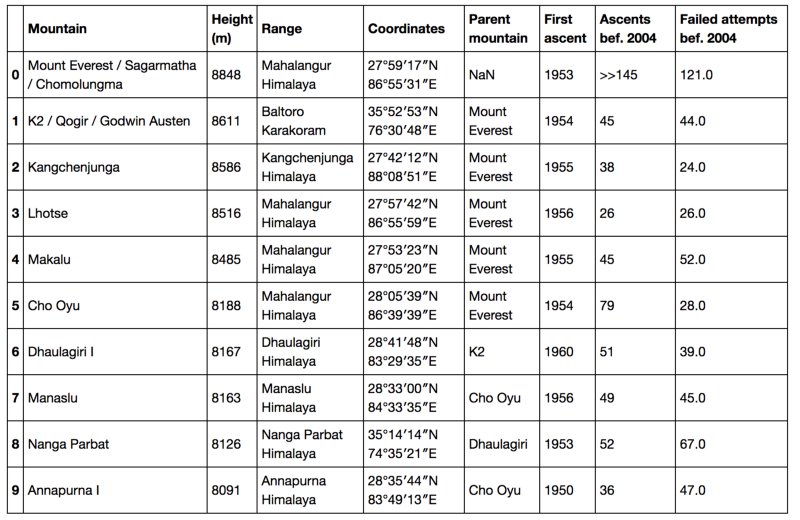
Dataframes
Data-Based Economics
Year 2025-2026
2026-01-14
Tabular Data
DataFrame
- A DataFrame (aka a table) is a 2-D labeled data structure with columns
- each column has a specific type and a column name
- types: quantitative, qualitative (ordered, non-ordered, …)
- First column is special: the index
- first goal of an econometrician: constitute a good dataframe
- aka “cleaning the data”
DataFrames are everywhere
- sometimes data comes from several linked dataframes
- relational database
- can still be seen conceptually as one dataframe…
- … through a join operation
- dataframes / relational databases are so ubiquitous a language has been developed for them
- SQL
- in the 80s…
- probably worth looking at if you have some “data” ambitions
- you will see the shadow of SQL everywhere - words like: join, merge, select, insert…
- plenty of resources to learn (example: sqbolt)
Pandas

pandas
- pandas = panel + datas
- a python library created by WesMcKinney
- very optimized
- essentially a dataframe object
- many options but if in doubt:
- minimally sufficient pandas is a small subset of pandas to do everything
- tons of online tutorials
creating a dataframe (1)
creating a dataframe (2)
- there are many other ways to create a dataframe
- for instance using a numpy matrix (numpy is a linear algebra library)
| age | travel | |
|---|---|---|
| 0 | 18 | 150 |
| 1 | 21 | 200 |
| 2 | 29 | 1500 |
File Formats
Common file formats
- comma separated files:
csvfile- often distributed online
- can be exported easily from Excel or LibreOffice
- stata files: use
pd.read_dta() - excel files: use
pd.read_excel()orxlsreaderif unlucky- note that excel does not store a dataframe (each cell is potentially different)
- postprocessing is needed
Comma separated file
- one can actually a file from python
- and import it
| year | country | measure | |
|---|---|---|---|
| 0 | 2018 | france | 950.0 |
| 1 | 2019 | france | 960.0 |
| 2 | 2020 | france | 1000.0 |
| 3 | 2018 | usa | 2500.0 |
| 4 | 2019 | usa | 2150.0 |
| 5 | 2020 | usa | 2300.0 |
“Annoying” Comma Separated File
- Sometimes, comma-separated files, are not quite comma-separated…
- inspect the file with a text editor to see what it contains
- the kind of separator, whether there are quotes…
- inspect the file with a text editor to see what it contains
- add relevant options to
pd.read_csvand check result
| year | country | measure | |
|---|---|---|---|
| 0 | 2018 | france | 950.0 |
| 1 | 2019 | france | 960.0 |
| 2 | 2020 | france | 1000.0 |
| 3 | 2018 | usa | 2500.0 |
| 4 | 2019 | usa | 2150.0 |
| 5 | 2020 | usa | 2300.0 |
Exporting a DataFrame
pandas can export to many formats:
df.to_...to (standard) CSV
,year,country,measure
0,2018,france,950.0
1,2019,france,960.0
2,2020,france,1000.0
3,2018,usa,2500.0
4,2019,usa,2150.0
5,2020,usa,2300.0- or to stata
Data Sources
Types of Data Sources
- Where can we get data from ?
- check one of the databases lists kaggle, econ network
- Official websites
- often in csv form
- unpractical applications
- sometimes unavoidable
- open data trend: more unstructured data
- Data providers
- supply an API (i.e. easy to use function)
Data providers
- commercial ones:
- bloomberg, macrobond, factsets, quandl …
- free ones available as a python library
dbnomics: many official time-seriesqeds: databases used by quanteconvega-datasets: distributed with altair
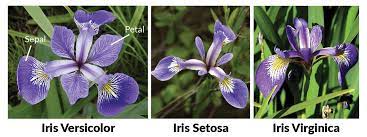
| sepalLength | sepalWidth | petalLength | petalWidth | species | |
|---|---|---|---|---|---|
| 0 | 5.1 | 3.5 | 1.4 | 0.2 | setosa |
| 1 | 4.9 | 3.0 | 1.4 | 0.2 | setosa |
| 2 | 4.7 | 3.2 | 1.3 | 0.2 | setosa |
| 3 | 4.6 | 3.1 | 1.5 | 0.2 | setosa |
| 4 | 5.0 | 3.6 | 1.4 | 0.2 | setosa |
| … | … | … | … | … | … |
| 145 | 6.7 | 3.0 | 5.2 | 2.3 | virginica |
| 146 | 6.3 | 2.5 | 5.0 | 1.9 | virginica |
| 147 | 6.5 | 3.0 | 5.2 | 2.0 | virginica |
| 148 | 6.2 | 3.4 | 5.4 | 2.3 | virginica |
| 149 | 5.9 | 3.0 | 5.1 | 1.8 | virginica |
150 rows × 5 columns
DBnomics example
- DBnomics aggregates time series from various public sources
- data is organized as provider/database/series
- try to find the identifer of one or several series
- tip: in case one python package is missing, it can be installed on the fly as in
Inspect / describe data
Inspecting data
- once the data is loaded as
df, we want to look at some basic properties: - general
df.head(5)# 5 first linesdf.tail(5)# 5 first linesdf.describe()# general summary
- central tendency
df.mean()# averagedf.median()# median
- spread
df.std()# standard deviationsdf.var()# variancedf.min(),df.max()# bounds
- counts (for categorical variable
- df.count()
| sepalLength | sepalWidth | petalLength | petalWidth | species | |
|---|---|---|---|---|---|
| 0 | 5.1 | 3.5 | 1.4 | 0.2 | setosa |
| 1 | 4.9 | 3.0 | 1.4 | 0.2 | setosa |
| sepalLength | sepalWidth | petalLength | petalWidth | |
|---|---|---|---|---|
| count | 150.000000 | 150.000000 | 150.000000 | 150.000000 |
| mean | 5.843333 | 3.057333 | 3.758000 | 1.199333 |
| std | 0.828066 | 0.435866 | 1.765298 | 0.762238 |
| min | 4.300000 | 2.000000 | 1.000000 | 0.100000 |
| 25% | 5.100000 | 2.800000 | 1.600000 | 0.300000 |
| 50% | 5.800000 | 3.000000 | 4.350000 | 1.300000 |
| 75% | 6.400000 | 3.300000 | 5.100000 | 1.800000 |
| max | 7.900000 | 4.400000 | 6.900000 | 2.500000 |
Manipulating DataFrames
Changing names of columns
- Columns are defined by property
df.columns
Index(['sepalLength', 'sepalWidth', 'petalLength', 'petalWidth', 'species'], dtype='object')- This property can be set with a list of the right length
| sLength | sWidth | pLength | pWidth | species | |
|---|---|---|---|---|---|
| 0 | 5.1 | 3.5 | 1.4 | 0.2 | setosa |
| 1 | 4.9 | 3.0 | 1.4 | 0.2 | setosa |
Indexing a column
- A column can be extracted using its name as in a dictionary (like
df['sLength'])
0      3.5
1      3.0
      ...
148    3.4
149    3.0
Name: sWidth, Length: 150, dtype: float64- The result is a series object (typed values with a name and an index)
- It has its own set of methods
- try:
series.mean(),series.std()series.plot()series.diff()- creates \(y_t = x_t-x_{t-1}\)
series.pct_change()- creates \(y_t = \frac{x_t-x_{t-1}}{x_{t-1}}\)
- try:
Creating a new column
- It is possible to create a new column by combining existing ones
| sLength | sWidth | pLength | pWidth | species | totalLength | |
|---|---|---|---|---|---|---|
| 0 | 5.1 | 3.5 | 1.4 | 0.2 | setosa | 6.5 |
| 1 | 4.9 | 3.0 | 1.4 | 0.2 | setosa | 6.3 |
Replacing a column
- An existing column can be replaced with the same syntax.
| sLength | sWidth | pLength | pWidth | species | totalLength | |
|---|---|---|---|---|---|---|
| 0 | 5.1 | 3.5 | 1.4 | 0.2 | setosa | 3.95 |
| 1 | 4.9 | 3.0 | 1.4 | 0.2 | setosa | 3.85 |
Selecting several columns
- Index with a list of column names
| pLength | sLength | |
|---|---|---|
| 0 | 1.4 | 5.1 |
| 1 | 1.4 | 4.9 |
| 2 | 1.3 | 4.7 |
Selecting lines (1)
- use index range
- ☡: in Python the end of a range is not included !
| sLength | sWidth | pLength | pWidth | species | totalLength | |
|---|---|---|---|---|---|---|
| 2 | 4.7 | 3.2 | 1.3 | 0.2 | setosa | 3.65 |
| 3 | 4.6 | 3.1 | 1.5 | 0.2 | setosa | 3.80 |
Selecting lines (2)
- let’s look at unique species
array(['setosa', 'versicolor', 'virginica'], dtype=object)- we would like to keep only the lines with
virginica
- the result is a boolean series, where each element tells whether a line should be kept or not
- if you want you can keep the recipe:
df[df['species'] == 'virginica']- to keep lines where
speciesis equal tovirginica
| sLength | sWidth | pLength | pWidth | species | totalLength | |
|---|---|---|---|---|---|---|
| 100 | 6.3 | 3.3 | 6.0 | 2.5 | virginica | 9.15 |
| 101 | 5.8 | 2.7 | 5.1 | 1.9 | virginica | 8.00 |
| 102 | 7.1 | 3.0 | 5.9 | 2.1 | virginica | 9.45 |
| 103 | 6.3 | 2.9 | 5.6 | 1.8 | virginica | 8.75 |
Selecting lines and columns
- sometimes, one wants finer control about which lines and columns to select:
- use
df.loc[...]which can be indexed as a matrix
- use
0    setosa
1    setosa
2    setosa
3    setosa
4    setosa
Name: species, dtype: object
Combine everything
- Here is an example combiing serveral techniques
- Let’s change the way totalLength is computed, but only for ‘virginica’
Reshaping DataFrames
The following code creates two example databases.
71136Wide vs Long format (1)
Compare the following tables
Wide vs Long format (2)
- in long format: each line is an independent observation
- two lines may belong to the same category (year, or country)
- all values are given in the same column
- their types/categories are given in another column
- in wide format: some observations are grouped
- in the example it is grouped by year
- values of different kinds are in different columns
- the types/categories are stored as column names
- both representations are useful
Tidy data:
- tidy data:
- every column is a variable.
- every row is an observation.
- every cell is a single value.
- a very good format for:
- quick visualization
- data analysis
Converting from Wide to Long
| year | variable | value | |
|---|---|---|---|
| 0 | 2018 | france | 950.0 |
| 1 | 2019 | france | 960.0 |
| 2 | 2020 | france | 1000.0 |
| 3 | 2018 | usa | 2500.0 |
| 4 | 2019 | usa | 2150.0 |
| 5 | 2020 | usa | 2300.0 |
Converting from Long to Wide
| measure | ||
|---|---|---|
| country | france | usa |
| year | ||
| 2018 | 950.0 | 2500.0 |
| 2019 | 960.0 | 2150.0 |
| 2020 | 1000.0 | 2300.0 |
| country | france | usa |
|---|---|---|
| year | ||
| 2018 | 950.0 | 2500.0 |
| 2019 | 960.0 | 2150.0 |
| 2020 | 1000.0 | 2300.0 |
groupby
groupbyis a very powerful function which can be used to work directly on data in the long format.- for instance to compute averages per country
| year | measure | |
|---|---|---|
| country | ||
| france | 2019.0 | 970.000000 |
| usa | 2019.0 | 2316.666667 |
- You can perform several aggregations at the same time:
Merging
Merging two dataframes
- Suppose we have two dataframes, with related observations
- How can we construct one single database with all informations?
- Answer:
concatif long formatmergedatabases if wide format
- Lots of subtleties when data gets complicated
- we’ll see them in due time
Merging two DataFrames with pandas
| year | country | measure | recipient | |
|---|---|---|---|---|
| 0 | 2018 | france | 950.0 | maxime |
| 1 | 2019 | france | 960.0 | mauricette |
| 2 | 2020 | france | 1000.0 | mathilde |
| 3 | 2018 | usa | 2500.0 | sherlock |
| 4 | 2019 | usa | 2150.0 | watson |
| 5 | 2020 | usa | 2300.0 | moriarty |