Real Business Cycles, with Dolo
Advanced Macro: Numerical Methods, 2021 (MIE37)
- Like the neo-classical growth model
- With shocks
- With labour
- With a decentralized interpretation
The RBC Model: planner version
states:
- productivity: \(z_t\)
- capital: \(k_t\)
two independent control variables:
- consumption: \(c_t \in [0,y_t], c_t\geq 0, c_t\leq y_t\)
- labor: \(n_t\)
shock:
- tfp shock: \(\epsilon_t \sim \mathcal{N}(0,\sigma)\)
objective: \[\max_{\begin{matrix}c_t, n_t\\\\c_t \geq 0, y_t \geq c_t, n_t \geq 0, 1 \geq n_t\end{matrix}} \mathbb{E}_0 \left[ \sum \beta^t \left( U(c_t) + \chi V(1-n_t) \right) \right]\]
U and V satisfy Inada conditions, ie \(U^{\prime}>0, U^{\prime \prime}<0, U^{\prime}(0)=\infty\)
- definitions:
- production: \[y_t = \exp(z_t) k_t^{\alpha} n^{1-\alpha} + i_t\]
- investment: \[i_t = y_t - c_t\]
- transitions: \[\begin{eqnarray} z_t = (1-\rho) z_{t-1} + \epsilon_t\\\\ k_t = (1-\delta) k_{t-1} + i_{t-1} \end{eqnarray}\]
Lagrangian
- Two variables optimization: \[\max_{\begin{matrix}c_1, c_2\\\\p_1 c_1 + p_2 c_t \leq B\end{matrix}} U(c_1, c_2)\]
- Deterministic opimization (finite horizon) \[\max_{\begin{matrix}c_0, c_1, c_2, ... c_T \\\\ c_0 + c_1 + \cdots + c_T \leq B\\\\c_0\geq0, \cdots c_T \geq 0 \end{matrix}} \sum_{i=1}^{T} \beta^i U(c_i)\]
- Deterministic opimization (infinite horizon) \[\max_{\begin{matrix}c_0, c_1, ... \\\\ c_0 + c_1 + \cdots \leq B\\\\c_0\geq0, c_1\geq 0, \cdots \end{matrix}} \sum_{i=1}^{\infty} \beta^i U(c_i)\]
Lagrangian (stochastic)
- exogenous process defines an event tree \((s)\)
- it is a very useful concept to understand stochastic optimization, complete markets, etc.
- math for continuous processes a bit involved (filtrations, …), but most intuition can be gained from discrete process
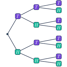
- consider a discrete process (for instance \(\epsilon_t \in [ \overline{\epsilon}, \underline{\epsilon}]\))
- an event is defined as the history of the shocks so far
- ex: \((\overline{\epsilon} , \overline{\epsilon}, \underline{\epsilon}, \overline{\epsilon})\)
- if \(s^{\prime}\) is the sucessor of \(s\) we denote \(s \subset s^{\prime}\)
- \(s\) is in the history of \(s^{\prime}\)
- transition probabilities \(\tau(s,s^{\prime})\)
- \(1 = \sum_{s^{\prime} | s\subset s^{\prime}} \tau(s, s^{\prime})\)
- each node has a given probability \(p(s)\). By construction:
- \(p(s^{\prime}) = p(s) \tau(s,s^{\prime})\)
- sometimes, we keep time subscript:
- ex: \(s_4 = (\overline{\epsilon} , \overline{\epsilon}, \underline{\epsilon}, \overline{\epsilon})\)
- but for each \(t\) there are many possible \(s_t\)
Lagrangian (stochastic 2)
Stochastic optimization (infinite horizon) \[\max_{ c_t } \mathbb{E_0} \left[ \sum_{t=1}^{\infty} \beta^i U(c_t) \right]\]
What it really means (\(|s|\) is time of event \(s\)) \[\max_{ \forall s, c(s)} \sum_{s} p(s) \beta^{|s|} U(c(s))\]
Or: \[\max_{ c(s_t) } \sum_{t} \beta^{t} \sum_{s_t} p(s_t)U(c(s_t))\]
Think of it as a regular sum
When you differentiate the lagrangian, you are differentiating w.r.t. all \(c(s_t)\), i.e the values of \(c\) on each of the nodes.
Example: cake eating
Back to RBC
\[\max_{\begin{matrix}c_t, n_t\\\\c_t \geq 0\\\\ y_t \geq c_t\\\\n_t \geq 0\\\\1 \geq n_t\end{matrix}} \mathbb{E}_0 \left[ \sum \beta^t \left( U(c_t) + \chi V(1-n_t) \right) \right]\]
- We know that optimally \(c_t>0\), \(c_t<y_t\) and \(n_t>0\)
- equality cases lead to zero production, i.e. infinite marginal utility
Back to RBC (2)
\[\max_{\begin{matrix}c_t, n_t\\\\c_t \geq 0\\\\ k_{t+1} \geq 0 \\\\n_t \geq 0\\\\1 \geq n_t \\\\ y_t \geq c_t - i_t \\\\ k_{t+1} = (1-\delta) k_t + i_t \\\\ y_t = e^{z_t} k_t^{\alpha} n_t^{1-\alpha} \end{matrix}} \mathbb{E}_0 \left[ \sum_t \beta^t \left( U(c_t) + \chi V(1-n_t) \right) \right]\]
- We know that optimally \(c_t>0\), and \(n_t>0\), \(k_{t+1}>0\)
- equality cases lead to zero production, i.e. infinite marginal utility
- we can drop the corresponding constraints
- We assume \(n_t=1\) is never binding (this would correspond to unemployment)
Back to RBC (3)
\[\mathcal{L} = \mathbb{E}\_0 \left[ \sum_t \beta^t \left\\{ \begin{matrix} U(c_t) + \chi V(1-n_t) \\\\ + \lambda_t (y_t - c_t) \\\\ + q_t (k\_{t+1} - (1-\delta) k_t - i_{t} ) \\\\ + \nu_t (y_t - e^{z_t} k_t^{\alpha}n_t^{1-\alpha}) \end{matrix} \right\\} \right]\]
- Let’s derive w.r.t. all nonpredetermined values within the sum:
- … explain
RBC first order conditions:
\[\begin{eqnarray} U^{\prime}(c_t) & = & \beta \mathbb{E}\_t \left[ U^{\prime} (c_{t+1}) \left( (1-\delta) + \alpha e^{z\_{t+1}} k\_{t+1}^{\alpha-1} n\_{t+1}^{1-\alpha} \right) \right] \\\\ \chi V^{\prime} (1-n_t) & = & (1-\alpha) e^{z_t} k_t^{\alpha} (n_t)^{-\alpha} U^{\prime}(c_t) \end{eqnarray}\]
Exercise:
- Set \(U(x) = \frac{c_t^{1-\gamma}}{1-\gamma}\), \(V(x) = \frac{(1-x)^{1-\eta}}{1-\eta}\)
- Try to find the steady state
- it is impossible to do so in closed-form
- Set \(\overline{n} = 0.33\) and adjust \(\chi\) so that it is a steady-state
The decentralized story
Planner vs decentralized
- So far, we have assumed, that the same agent decides on consumption and labour supply
- What if some decisions are taken in some decentralized markets?
- New structure:
- decentralized competitive firms
- rent capital and workers
- sell goods
- a representative household
- supplies labour
- accumulates capital and rents it to firms
- consume goods
- decentralized competitive firms
The firms
- Firm \(i\)
- chooses capital \(k^i\) and labour \(n^i\)
- Cobb Douglas production: \(y_i = f(k_i, n_i) = (k_i)^{\alpha} (n_i)^(1-\alpha)\)
- Since there is only one good, its price can be set to \(1\)
- Firm takes wages \(w\) and rental price of capital \(r\) as given: \[max_{k_i, n_i} \pi(k_i, n_i) = f(k_i, n_i) - r k_i - w n_i\]
- Optimally:
- \(f_k^{\prime}(k_i, n_i) = \alpha k_i^{\alpha-1} n_i^{1-\alpha} = r\)
- \(f_n^{\prime}(k_i, n_i) = (1-\alpha) k_i^{\alpha-1} n_i^{-\alpha} = w\)
- Remark:
- capital share: \(\frac{r k_i}{y_i} = \alpha\)
- labour share: \(\frac{w n_i}{y_i} = 1- \alpha\)
- profits are zero
Aggregation
- What is the production of all firms if total capital is \(K\) and total labour is \(L\) ?
- Note that for each firm \[(1 - \alpha) \frac{k_i}{l_i} = \alpha \frac{w}{r}\]
- We can sum over all firms to get: \[(1-\alpha){K} = \alpha \frac{w}{r}L\]
- we can write: \[y_i = (k_i)^{\alpha} (n_i)^{1-\alpha} = k_i \left( \frac{k_i}{n_i} \right)^{1-\alpha} = k_i (K/L)^{1-\alpha}\]
- and sum over all firms: \[Y = K (K/L)^{1-\alpha} = K^\alpha L ^{1-\alpha}\]
- The sum of many cobb douglas-firms is a big cobb-douglas firm !
Representative agent
- Our representative agent takes \(w_t\) and \(r_t\) as given.
- He supplies labour and capital, and decides how much to save so as to maximize: \[\max_{\begin{matrix} c_t, n_t \\\\ c_t \leq \pi_t + r_t k_t + w_t n_t - i_t \\\\ k_{t+1} = (1-\delta) k_t + i_t \\\\ c_t \geq 0 \end{matrix}} \sum_t \beta^t \left(U(c_t) + V(n_t) \right)\]
- Result: \[\begin{eqnarray} \beta U^{\prime}(c_t) & = & \beta \mathbb{E}\_t \left[ U^{\prime} (c_{t+1}) \left( (1-\delta) + r_{t+1}\right) \right] \\\\ \chi V^{\prime} (1-n_t) & = & w_t U^{\prime}(c_t) \end{eqnarray}\]
-
Result:
- exactly the same equations as in the central planner version (in this case)
- this formulation can be used to study distortionary taxes:
- ex: labour income tax \(\tau\)
Labour tax
- Our representative agent takes \(w_t\) and \(r_t\) as given.
- He supplies labour and capital, and decides how much to save so as to maximize: \[\max_{\begin{matrix} c_t, n_t \\\\ c_t \leq \pi_t + (1-\tau) w_t n_t + r_t k_t - i_t + g_t \\\\ k_{t+1} = (1-\delta) k_t + i_t \\\\ c_t \geq 0 \end{matrix}} \sum_t \beta^t \left(U(c_t) + V(n_t) \right)\]
- Note the new budget constraint
- labour income is taxed, but a lump-sum subsidy ensures nothing is destroyed
- \(g_t =\tau w_t k_t\) is not taken into account for intertemporal optimization
- Result: \[\begin{eqnarray} \beta U^{\prime}(c_t) & = & \beta \mathbb{E}\_t \left[ U^{\prime} (c_{t+1}) \left( (1-\delta) + r_{t+1}\right) \right] \\\\ \chi V^{\prime} (1-n_t) & = & (1-\tau) w_t U^{\prime}(c_t) \end{eqnarray}\]
-
Result:
- exactly the same equations as in the central planner version (in this case)
- this formulation can be used to study distortionary taxes:
- ex: labour income tax \(\tau\)