Time Iteration
Advanced Macro: Numerical Methods
2025-04-17
Approximate Dynamic Programming
What’s new today?
- The nature of the problem:
- Last time we did discrete dynamic programming: \(S\) and \(X\) finite
- Today both are continuous: approximate dynamic programming
- today, we have continuous decision rules
- we will need to discretize and interpolate
- The representation of the model
- We used the Bellman representation
- Today we use first order representation (Euler and co.)
- The solution metod:
- We will see the main time-iteration algorithms
First order representation of a model
What’s new today?
- A few weeks ago, we did discrete dynamic programming
- today, we have continuous decision rules
- we will need to interpolate
- We were using Bellman representation
- we’ll use first order representation (Euler and co.)
- We will see the main time-iteration algorithms
- and mention some of its variants
Generic Value Function Representation
- All variables of the model are vectors:
- states \(s \in \mathcal{S} \subset R^{n_s}\)
- controls \(x \in \mathcal{F}(\mathcal{S}, R^{n_x})\)
- we assume bounds \(a(s)\leq x \leq b(s)\)
- shocks: \(\epsilon \sim \text{i.i.d. distrib}\)
- Transition: \[s_{t+1} = g(s_t, x_t, \epsilon_{t+1})\]
- Value function: \[V(s) = E_0 \sum_{t\geq 0} \beta^t \left[ U(s_t, x_t)\right]\]
- Solution is a function \(V()\) (value) which is a fixed point of the Bellman-operator: \[\forall s, V(s) = \max_{a(s)\leq x \leq b(s)} U(s,x) + \beta E \left[ V(g(s,x,\epsilon)) \right]\]
- The argmax, defines a decision rule function: \(x = \varphi(s)\)
First order representation
- All variables of the model are vectors:
- states \(s_t\)
- controls \(x_t\)
- we assume bounds \(a(s)\leq x \leq b(s)\)
- shocks: \(\epsilon_t\) (i.i.d. random law)
- Transition: \[s_{t+1} = g(s_t, x_t, \epsilon_{t+1})\]
- Decision rule: \[x_t = \varphi(s_t)\]
- Arbitrage: \[ E_t\left[ f(s_t, x_t, s_{t+1}, x_{t+1}) \right] = 0 \perp a(s_t) \leq x_t \leq b(s_t) \]
- These equations must be true for any \(s_t\).
- Remark: time subscript are conventional. They are used to precise:
- when expectation is taken (w.r.t \(\epsilon_{t+1}\))
- to avoid repeating \(x_t=\varphi(s_t)\) and \(x_{t+1} = \varphi(s_t)\)
- Sometimes there are bounds on the controls
- we encode them with complementarity constraints
- more on it later
Example 1: neoclassical growth model
- capital accumulation: \[k_t = (1-\delta)k_{t-1} + i_{t-1}\]
- production: \[y_t = k_t^\alpha\]
- consumption: \[c_t = (1-s_t) y_t\] \[i_t = s_t y_t\]
- optimality: \[\beta E_t \left[ \frac{U^{\prime}(c_{t+1})}{U^{\prime}(c_{t})} (1-\delta + \alpha k_{t+1}^{\alpha-1}\alpha) \right]= 1\]
- states: \(k_t\), with one transition equation
- controls: \(y_t, c_t, i_t, s_t\), with four “arbitrage” equations
- it is possible but not mandatory to reduce the number of variables/equations by simple susbtitutions
Example 2: consumption-savings model
Simplest consumption/savings model:
- Transition: \[w_t = \exp(\epsilon_t) + (w_{t-1} - c_{t-1}) \overline{r}\]
- Objective: \[\max_{0\leq c_t \leq w_t} E_0 \left[ \sum \beta^t U(c_t) \right]\]
- First order conditions: \[\beta E_t \left[ \frac{U^{\prime}(c_{t+1})}{U^{\prime}(c_t)} \overline{r} \right] - 1 \perp 0 \leq c_t \leq w_t\]
F.O.C. reads as: \[\beta E_t \left[ \frac{U^{\prime}(c_{t+1})}{U^{\prime}(c_t)} \overline{r} \right] - 1 \leq 0 \perp c_t \leq w_t\] and \[0 \leq \beta E_t \left[ \frac{U^{\prime}(c_{t+1})}{U^{\prime}(c_t)} \overline{r} \right] - 1 \perp 0 \leq c_t \]
First one reads: if my marginal utility of consumption today is higher than expected mg. utility of cons. tomorrow, I’d like to consume more, but I can’t because, consumption is bounded by income (and no-borrowing constraint).
Second one reads: only way I could tolerate higher utility in the present, than in the future, would be if I want dissave more than I can, or equivalently, consume less than zero. This is never happening.
Example 3: new-keynesian with / without ZLB
Consider the new keynesian model we have seen in the introduction:
- Assume \(z_t\) is an autocorrelated shock: \[z_t = \rho z_{t-1} + \epsilon_t\]
- New philips curve (PC):\[\pi_t = \beta \mathbb{E}_t \pi_{t+1} + \kappa y_t\]
- dynamic investment-saving equation (IS):\[y_t = \beta \mathbb{E}_t y_{t+1} - \frac{1}{\sigma}(i_t - \mathbb{E}_t(\pi_{t+1}) ) - {\color{green} z_t}\]
- Interest Rate Setting (taylor rule): \[i_t = \alpha_{\pi} \pi_t + \alpha_{y} y_t\]
The model satisfies the same specification with:
- one state \(z_t\) and one transition equation
- three controls: \(\pi_t\), \(y_t\) and \(i_t\) with three “arbitrage” equation
These are not real first order conditions as they are not derived from a maximization program
- unless one tries to microfound them…
It is possible to add a zero-lower bound constraint by replacing IRS with: \[ \alpha_{\pi} \pi_t + \alpha_{y} y_t \leq i_t \perp 0 \leq i_t\]
Time iteration
Time iteration
- So we have the equation, \(\forall s_t\)
\[ E_t\left[ f(s_t, x_t, s_{t+1}, x_{t+1}) \right] = 0 \perp a(s_t) \leq x_t \leq b(s_t)\]\[ E_t\left[ f(s_t, x_t, s_{t+1}, x_{t+1}) \right] = 0\]where \[s_{t+1} = g(s_t, x_t, \epsilon_{t+1})\] \[x_t = \varphi(s_t)\] \[x_{t+1} = \tilde{\varphi}(s_{t+1})\]
- Let’s leave the complementarity conditions aside for now
- In equilibrium \(\tilde{\varphi} = {\varphi}\)
Time iteration
- We can rewrite everything as one big functional equation: \[\forall s, \Phi(\varphi, \tilde{\varphi})(s) = E\left[ f(s, \varphi(s), g(s,\varphi(s), \epsilon), \tilde{\varphi}(g(s,\varphi(s), \epsilon)) \right]\]
- A solution is \(\varphi\) such that \(\Phi(\varphi, \varphi) = 0\)
- The Coleman operator \(\mathcal{T}\) is defined implicitly by: \[\Phi(\mathcal{T}(\varphi), \varphi)=0\]
- The core of the time iteration algorithm, consists in the recursion: \[\varphi_{n+1} = \mathcal{T}(\varphi_n)\]
- It maps future decision rules to current decision rules
- same as “linear time iterations”, remember?
- Sounds fun but how do we implement it concretely?
Practical implementation
- We need to find a way to:
- compute expectations
- represent decision rules \(\varphi\) and \(\varphi\) with a finite number of parameters
Practical implementation (2)
- Computing expectations:
- discretize shock \(\epsilon\) with finite quantization \((w_i, e_i)_{i=1:K}\)
- replace optimality condition with: \[\forall s, \Phi(\varphi, \tilde{\varphi})(s) = \sum_i w_i f(s, \varphi(s), g(s,\varphi(s), e_i), \tilde{\varphi}(g(s,\varphi(s), e_i)) \]
- … but we still can’t compute all the \(\varphi\)
Approximating decision rules
- We’ll limit ourselves to interpolating functional spaces
- We define a finite grid \(\mathbf{s}=(s_1, ... s_N)\) to approximate the state space (\(\mathbf{s}\) is a finite vector of points)
- If we know the vector of values \(\mathbf{x}=(x_1, ..., x_N)\) a function \(\varphi\) takes on \(\mathbf{s}\), we approximate \(\varphi\) at any \(s\) using an interpolation scheme \(\mathcal{I}\): \[\varphi(s) \approx \mathcal{I}(s, \mathbf{s}, \mathbf{x})\]
- Now if we replace \(\varphi\) by \(\mathcal{I}(s, \mathbf{s}, \mathbf{x})\) and \(\tilde{\varphi}\) by \(\mathcal{I}(s, \mathbf{s}, \mathbf{\tilde{x}})\) the functional equation becomes: \[\forall s, \Phi(\varphi, \tilde{\varphi})(s) \approx F( \mathbf{x}, \mathbf{\tilde{x}} )(s) = \sum_i w_i f(s, x, \tilde{s}, \tilde{x})\] where \[x = \mathcal{I}(s, \mathbf{s}, \mathbf{x})\] \[\tilde{s} = g(s, x, e_i)\] \[\tilde{x} = \mathcal{I}(s, \mathbf{s}, \mathbf{\tilde{x}})\]
Pinning down decision rules
- Note that this equation must be statisfied \(\forall s\).
- In order to pin-down the \(N\) coefficients \(\mathbf{x}\), it is enough to satisfy the equations at \(N\) different points.
- Hence we solve the square system: \[\forall i\in [1,N], F( \mathbf{x}, \mathbf{\tilde{x}} )(s_i) = 0\]
- In vectorized form, this is just: \[F( \mathbf{x}, \mathbf{\tilde{x}} )(\mathbf{s}) = 0\]
- Or, since grid \(\mathbf{s}\) is fixed: \[F( \mathbf{x}, \mathbf{\tilde{x}} ) = 0\]
- Now the vector of decisions today, at each point of the grid, is determined as a function of the vector of decisions tomorrow, on the same grid.
Recap
- Choose a finite grid for states \(\mathbf{s} = (s_1, ..., s_N)\)
- For a given vector of controls tomorrow \(\mathbf{\tilde{x}}\), one can compute theoptimality of a vector of controls today by computing the value of :\[F( \mathbf{x}, \mathbf{\tilde{x}} ) = \sum_i w_i f(\mathbf{s}, \mathbf{x}, \tilde{\mathbf{s}}, \tilde{\mathbf{x}})\] \[\mathbf{\tilde{s}} = g(\mathbf{s}, \mathbf{x}, e_i)\] \[\mathbf{\tilde{x}} = \mathcal{I}(\mathbf{\tilde{s}}; \mathbf{s}, \mathbf{{x}})\]
- Note that because we use interpolating approximation: \(\forall i, x_i = \mathcal{I}(s, \mathbf{s}, \mathbf{x})\)
- We have enough to define an approximated time-iteration operator: implicitly defined by \[F(T(\mathbf{x}), \mathbf{x}))\]
- We can then implement time-iteration, but…
- how do we compute \(T(x)\)?
Computing \(T(\mathbf{x})\)
- In each step, we have a guess, for decision rule tomorrow \(\mathbf{\tilde{x}}\)
- We can then find the decision rule today, by solving numerically for: \(\mathbf{x} \mapsto F(\mathbf{x}, \mathbf{\tilde{x}})\)
- usually with some variant of a Newton method
- It is possible to solve for the values at each grid point separately…
- for each \(i\), find optimal controls \(x_i\) in state \(s_i\) that satisfy \(F(x_i, \mathbf{\tilde{x}}) = 0\)
- all the problems are independent from each other
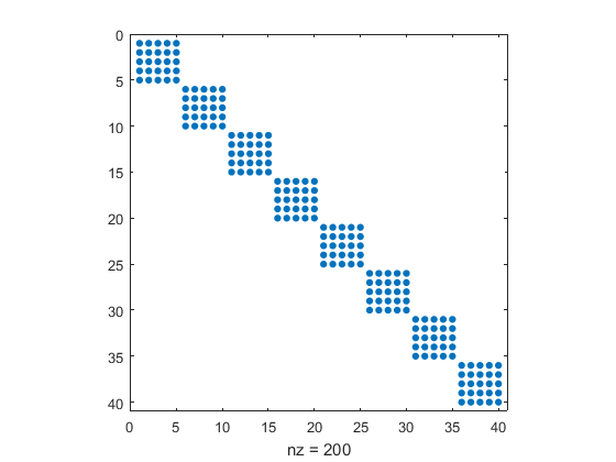
- …or to solve everything as a big system
- the jacobian is block-diagonal: finding optimal value in state \(i\) or in state \(j\) today are two independent problems
Time iteration algorithm
- Discretize state-space with grid \(\mathbf{s}=(s_1, ..., s_N)\)
- Choose initial values, for the vector of controls on the grid \(\mathbf{x}=(x_1, ..., x_N)\)
- Specify tolerance levels \(\eta>0\) and \(\epsilon>0\)
- Given an intial guess \(\mathbf{x_n}\)
- find the zero \(\mathbf{x_{n+1}}\) of function \(\mathbf{u}\mapsto F(u,\mathbf{x_n})\)
- that is, such that controls on the grid are optimal given controls tomorrow
- nonlinear solver can use \(\mathbf{x_n}\) as initial guess
- compute norm \(\mathbf{\eta_n} = |\mathbf{x_n} - \mathbf{x_{n+1}}|\)
- if \(\eta_n<\eta\), stop and return \(\mathbf{x_{n+1}}\)
- else, set \(\mathbf{x_n} \leftarrow \mathbf{x_{n+1}}\) and continue
- find the zero \(\mathbf{x_{n+1}}\) of function \(\mathbf{u}\mapsto F(u,\mathbf{x_n})\)
- Like usual, during the iterations, it is useful to look at \(\mathbf{\epsilon_n}=|F(\mathbf{x_n},\mathbf{x_n})|\) and \(\lambda_n = \frac{\eta_n}{\eta_{n-1}}\)
What about the complementarities ?
- When there aren’t any occasionally binding constraint, we look for the of zero \(\mathbf{x_{n+1}}\) of function \(\mathbf{u}\mapsto F(u,\mathbf{x_n})\).
- If we define the vector of constraints on all grid points as \(\mathbf{a}=(a(s_1), ..., a(s_N))\) and \(\mathbf{b}=(b(s_1), ..., b(s_N))\), we can rewrite the system to solve as: \[F(u) \perp \mathbf{a} \leq u \leq \mathbf{b}\]
- Then we can:
- feed \(F\), \(a\) and \(b\) to an NCP solver (like nlsolve.jl)
- or transform this relation using Fisher-Burmeister function into a smooth nonlinear system
Time iteration variants
You can check out:
- endogenous grid points:
- mathematically equivalent to TI,
- much faster for models that have a particular structure (consumption saving models)
- no need for a nonlinear solver
- improved time iterations:
- same as policy iterations for value function iterations
- convergence is equivalent to that of TI
- much faster but requires correct initial guess
- parameterized expectations
- requires that all controls are determined as a function of expectations
And Dolo.jl for a library that implements some of these algorithms.