Modélisation d’une petite économie ouverte
Modèle de dotation
L’agent représentatif maximise : \[\max_{c_t} \sum_{t=0}^{\infty} \beta^t u(c_t)\] \[c_t + a_{t} \leq y_t + (1+r) a_{t-1} \]
Économie de dotation :
- le revenu \((y_t)_t\) est donné de manière exogène
- par souci de simplicité, on suppose qu’il est déterministe
Petite économie ouverte :
- ouverte : peut épargner \(a_t\) ce qui rapporte \(a_{t+1}(1+r)\) à la période suivante
- petite : le pays considère le taux d’intérêt mondial \(r\) comme donné (pas d’effet sur les prix mondiaux)
Nous résolvons ce problème avec les conditions aux limites :
La condition de pas de Ponzi va effectivement éliminer les solutions divergentes.
Dans une approximation au premier ordre, elle sélectionne les bonnes valeurs propres.
Modèle de dotation (3)
Nous obtenons le Lagrangien :
\[\mathcal{L}= \sum_{t=0}^{\infty} \beta^t u(c_t) + \sum_{t=0}^{\infty} \beta^t \lambda_t \left(y_t + (1+r) a_{t-1} - c_t-a_{t} \right)\]
Conditions du premier ordre :
\[\begin{align}
u^{\prime}(c_t)& =& \lambda_t \\
\lambda_t &=& \beta (1+r) \lambda_{t+1}
\end{align}\]
Sous l’hypothèse technique \(\beta (1+r)=1\) nous obtenons \(c_t=c_{t+1}\) et donc
\[c_0 = \frac{r}{1+r}\left\{ (1+r) a_{-1} + \sum_{t=0}^{\infty} \frac{y_t}{(1+r)^t}\right\}\]
- la consommation est déterminée par le revenu permanent
- les changements de richesse initiale ont des effets permanents
- remarque : problème isomorphe aux décisions d’épargne-consommation
Compte courant
Rappels sur le compte courant
La balance commerciale est les exportations moins les importations (ici \(y_t-c_t\))
Le compte courant est la balance commerciale plus les revenus nets de facteurs (ici \(y_t-c_t+r a_{t-1}\))
Un compte courant positif : le pays prête au reste du monde.
En utilisant la formule d’avant
\[CA_0 = a_{-1} r + (1-\frac{r}{1+r}) y_0 - \frac{r}{1+r}\left\{ \sum_{t\geq1}^{\infty} \frac{y_t}{(1+r)^t}\right\}\]
Comment le compte courant réagit-il aux chocs de revenu ?
Racine unitaire
Reprenons la formule de la consommation : \[c_0 = \frac{r}{1+r}\left\{ (1+r) a_{-1} + \sum_{t=0}^{\infty} \frac{y_t}{(1+r)^t}\right\}\]
Rappelons aussi l’équation d’accumulation des actifs étrangers : \[a_t = (1+r) a_{t} + y_t - c_t\]
Lorsque \(a_{-1}\) augmente de \(\Delta a_{-1}\), alors \(c_0\) augmente de \(r \Delta a_{-1}\).
En conséqence \(a_0\) augmente d’exactement \(\Delta a_{-1}\) (car \(a_0 = (1+r) a_{-1} + y_0 - c_0\)).
En itérant le raisonnement, \(a_1, a_2, ...\) augmentent aussi d’exactement \(\Delta a_{-1}\).
Et les consomations \(c_1, c_2, ...\) augmentent d’exactement \(r \Delta a_{-1}\).
Une augmentation de la richesse initiale a un effet permanent sur les actifs étrangers et la consommation.
- cela correspondra à une racine unitaire dans la solution (valeur propre de module 1)
Ajout du capital
Nous ajoutons le capital et la production à notre économie de dotation : \[y_t = z_t k_{t-1}^\alpha\] \[k_t = (1-\delta) k_{t-1} + i_{t}\]
La contrainte de ressource agrégée devient :
\[a_{t} + c_t + i_t = (1+r) a_{t-1} + y_t\]
On maximise alors \(\sum_t \beta^ t U(c_t)\)
Nous obtenons les conditions du premier ordre (exactement comme dans le RBC)
\[\lambda_t = \beta \lambda_{t+1} (1+r)\] \[\lambda_t = \beta \lambda_{t+1}\left[ (1-\delta) + z_{t+1} f^{\prime}(k_{t}) \right]\]
où \(\lambda_t\) est le multiplicateur de Lagrange associé à la contrainte budgétaire.
Ajout du capital : conditions d’optimalité
Puisque \(\lambda_t>0\) (la contrainte est toujours active), nous obtenons :
\[(1-\delta) + z_{t+1} f^{\prime}(k_{t}) = 1+r\]
\[k_{t} = \left( \frac{r+\delta}{\alpha z_{t+1}}\right)^{\frac{1}{\alpha-1}}\]
et l’investissement \[i_t = \left( \frac{r+\delta}{\alpha z_{t+1}}\right)^{\frac{1}{\alpha-1}}- (1-\delta)\left( \frac{r+\delta}{\alpha z_{t}}\right)^{\frac{1}{\alpha-1}}\]
Ici l’investissement est entièrement déterminé par les chocs de productivité
⇒ trop simple :
- très corrélé avec la productivité
- pas de dépendance internationale
- ajustment immédiat du capital
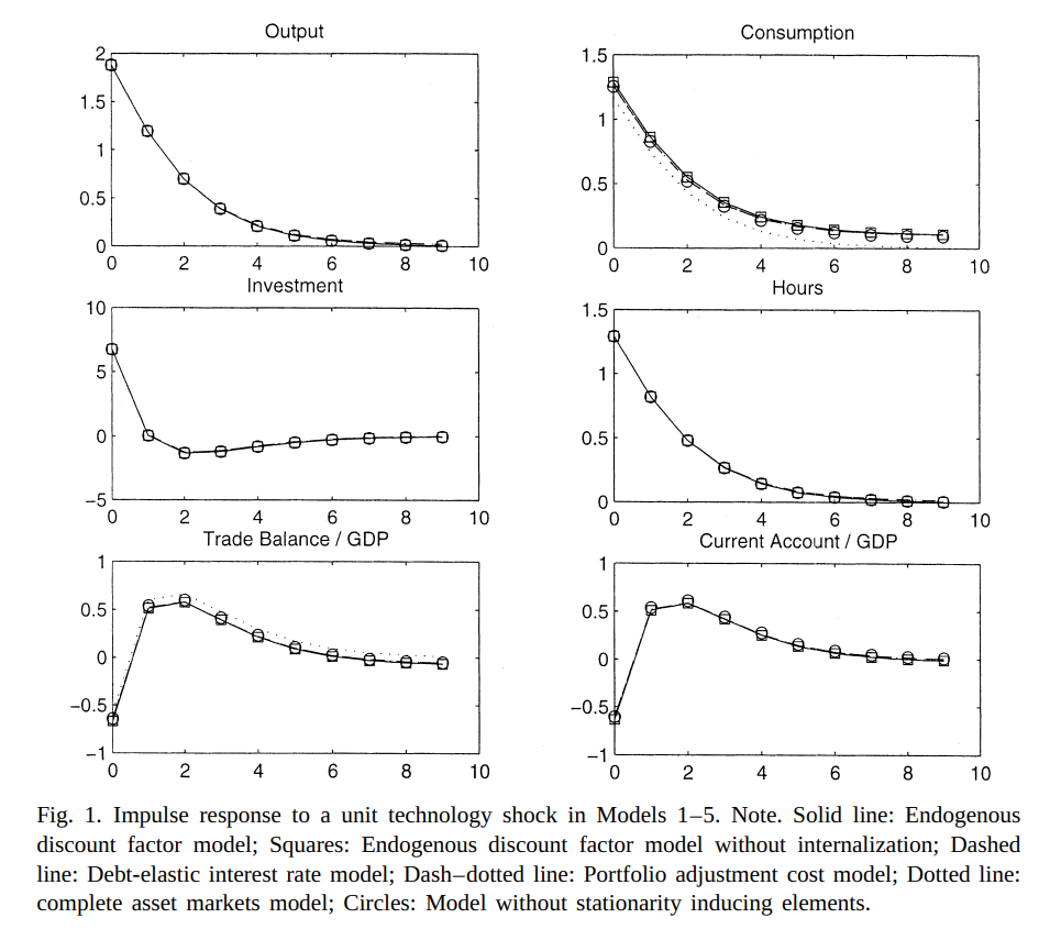
Ajout de frictions à l’investissement
Une solution possible : modifier la contrainte de ressource de sorte que l’ajustement du capital soit coûteux
Par exemple :
\[a_{t} + c_t + i_t + \frac{\omega}{2}\frac{(k_{t}-k_{t-1})^ 2}{k_t} = (1+r)a_{t-1} + z f(k_{t-1})\]
\[k_{t} = (1-\delta) k_{t-1} + i_t\]
où \(\omega\) est un paramètre de friction d’ajustement.
En général, \(\omega\) est choisi de sorte que le modèle reproduise \(\frac{Var(i_t)}{Var(y_t)}\) à partir des données.

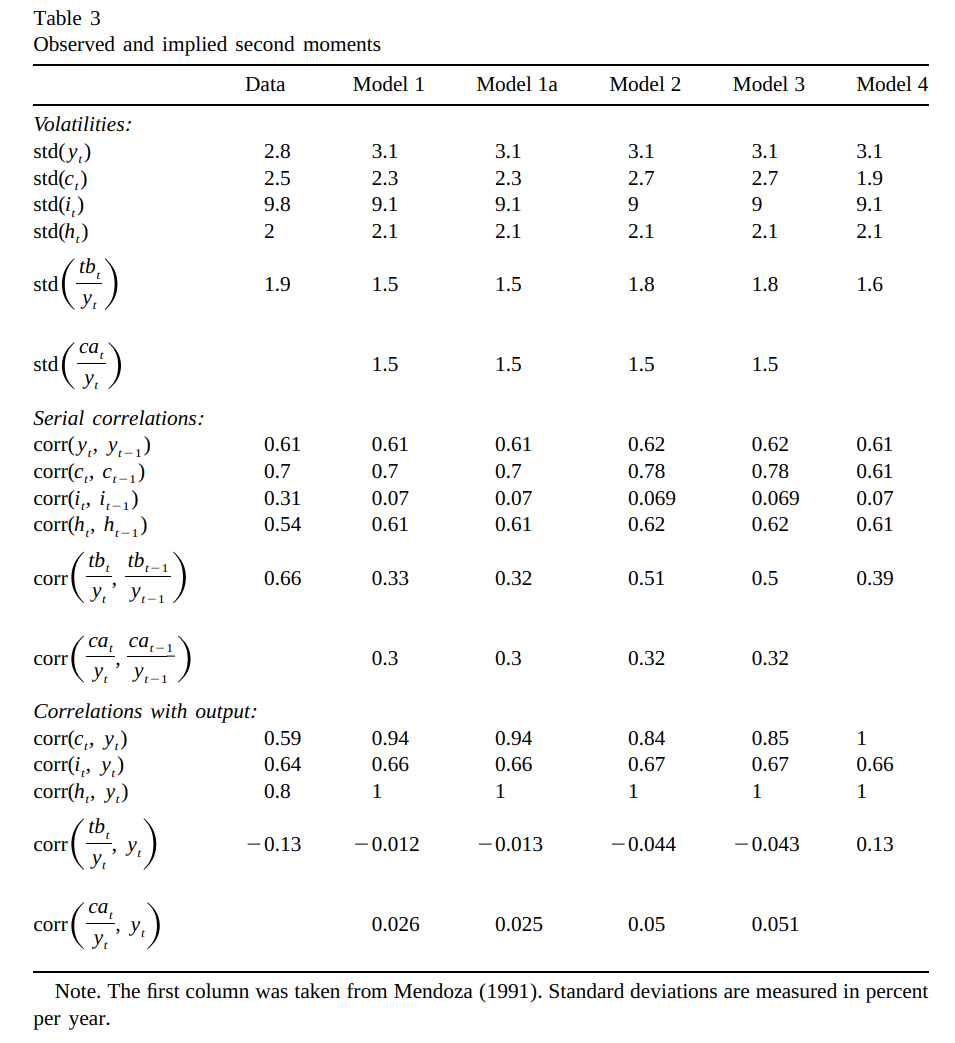
Comment rendre la distribution stationnaire ?
Sans \(\color{red}\pi\) la solution du modèle présente une racine unitaire :
\[a_t = a_{t-1} + ... \text{autres variables en t-1} + \text{chocs en t}\]
Problème :
Cela soulève des problèmes pratiques (notamment pour l’estimation) pour le modèle linéaire.