Discretization

Introduction

Several kinds of Discretization

  • approximate operator with a finite number of iterations:
    • compute \(\int_a^b f(x) dx\)
    • compute \(E_\omega f(\omega)\)
  • represent an infinite dimensional object with a finite set of parameters:
    • \(f \equiv (f(x_i))_{i=1:N}\) with \(x_i=a+\frac{i-1}{N-1}(b-a)\)
      • discretize arguments
    • \(\omega \equiv (\mu_i, \omega_i)_{i=1:N}\) such that \(E_\omega f(\omega) \approx \sum_i \mu_i f(\omega_i)\) (quantization)
  • discretize continous process by a discrete one:
    • continuous markov chain to discrete markov Chain

Discretizing an iid law

Common problem:

Given \(f\), and an iid process \(\epsilon \sim N(0,\sigma^2)\), how to approximate \(E_{\epsilon} f(\epsilon)\) ?

Some Ideas:

  • draw lots of random \((\epsilon_n)_{n=1:N}\) and compute \[\frac{1}{N}\sum_{n=1}^N f(\epsilon_n)\]
    • aka Monte-Carlo simulations
  • given a method to approximate integrals, define \(\mu(u)=\frac{1}{\sigma\sqrt{2 \pi}}e^{-\frac{u^2}{2\sigma^2}}\) and compute \[\int_{u=-\infty}^{\infty} f(u) \mu(u) du\]
  • discretize (or quantize) the signal \(\epsilon\) as \((w_i, \epsilon_i)_{i=1:N}\) and compute: \[\frac{1}{N} \sum_n w_n f(\epsilon_n)\]

What’s wrong with Monte-Carlo Simulations?

Define \(X(\epsilon) = U(C(\epsilon))\) where \(U(c)=\frac{c^{1-\gamma}}{1-\gamma}\) and \(C(\epsilon) = e^{\epsilon}\). We want to compute \(E_{\epsilon} X(\epsilon)\) precisely.

How many draws do we need ?

Monte Carlo estimate of E[X] versus number of draws in a 2x1 layout with empty second panel.

Monte Carlo estimate with plus/minus one standard deviation intervals and standard deviation decay versus number of draws in a 2x1 layout.

Monte Carlo estimate with plus/minus one standard deviation intervals and standard deviation decay versus number of draws in a 2x1 layout with logarithmic x-axis.

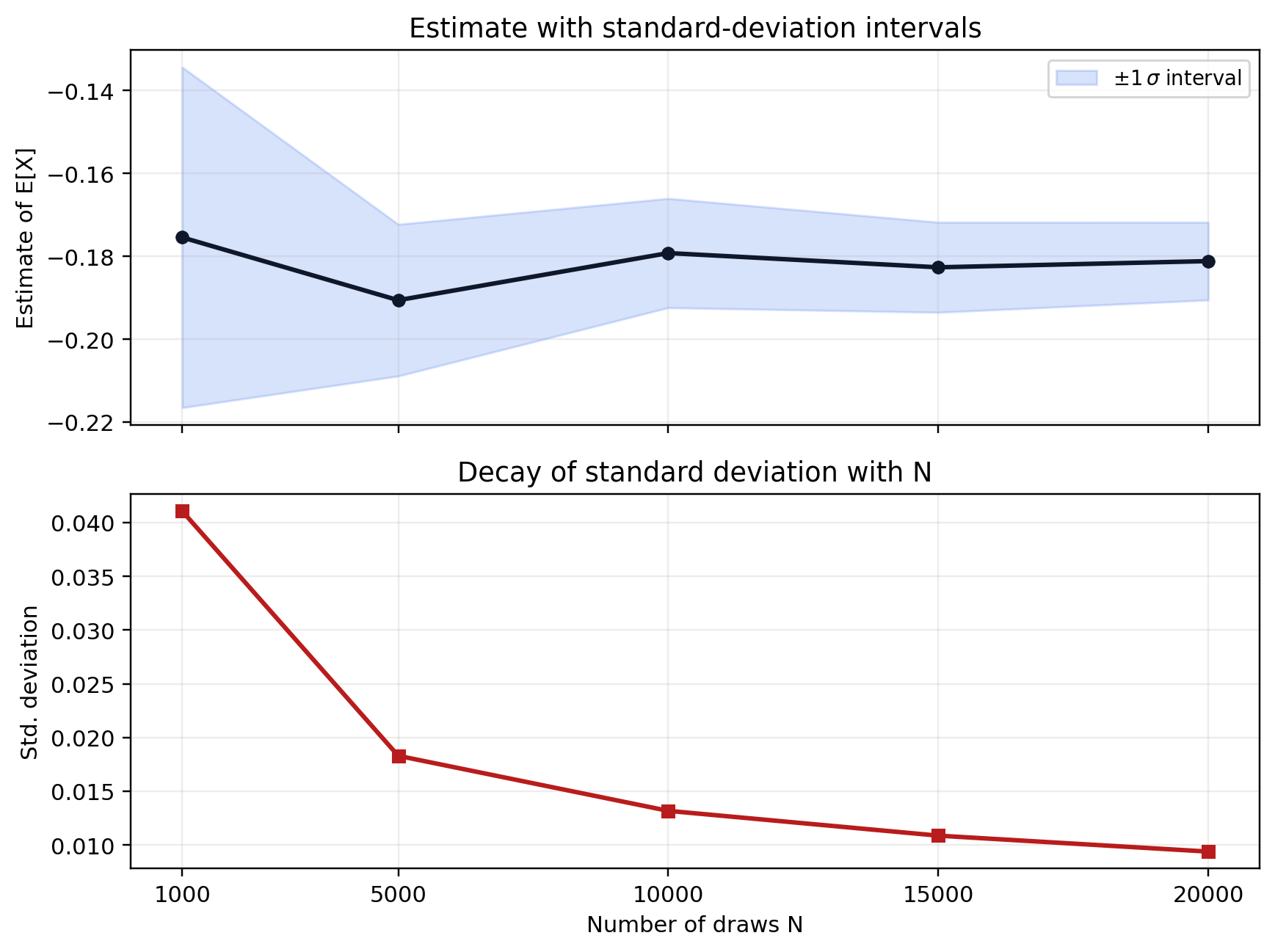
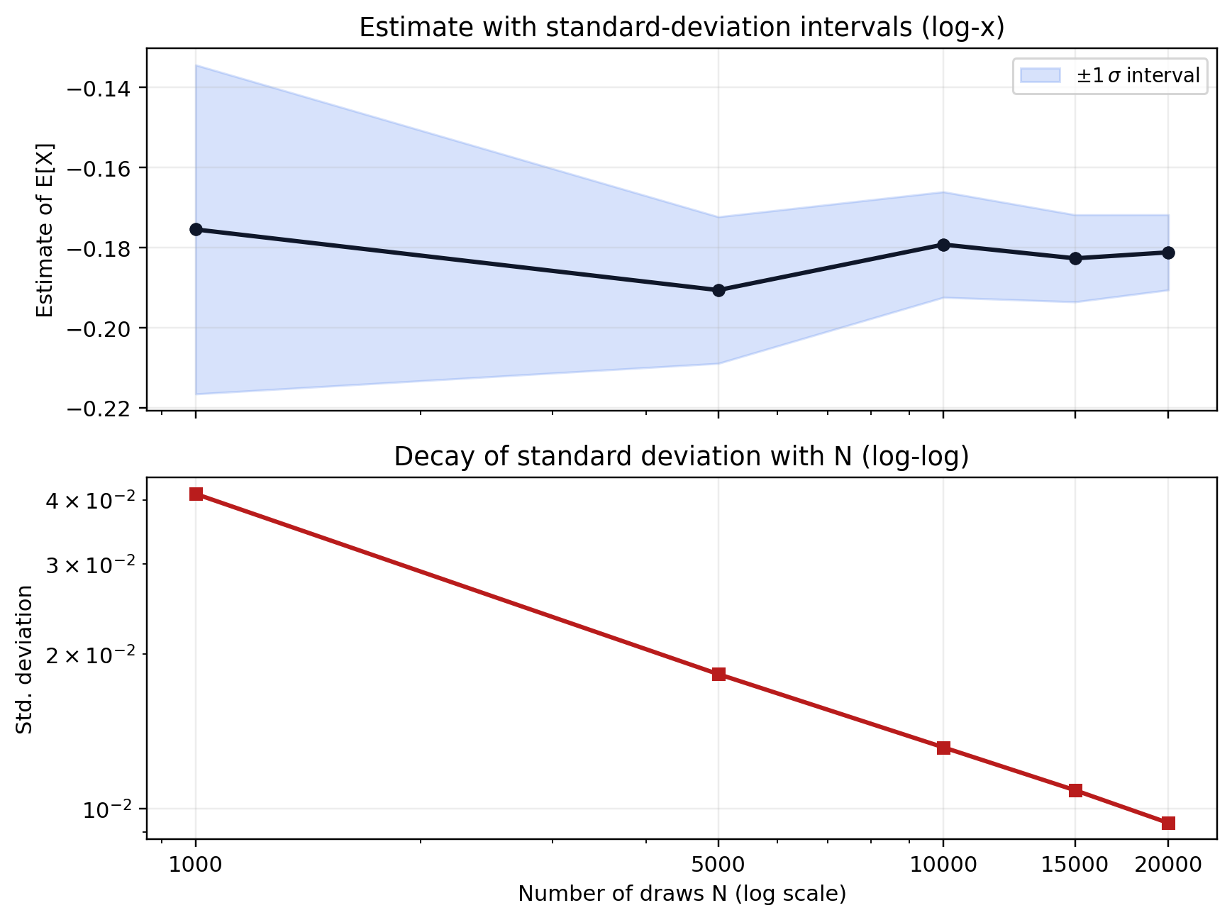
The decrease in standard deviations is too slow.

Define the Model in Julia

# imports:
using Distributions: Normal

# define the model
σ = 0.05; γ = 40
C(e) = exp(e)
U(x)=(x^(-γ))/(-γ)
X(e) = U(C(e))

# create distributions
dis = Normal(0,σ)      
E_ϵ(f;N=1000) = sum(f(rand(dis)) for i=1:N)/N

NVec = [1000, 5000, 10000, 15000, 20000]

Monte-Carlo estimates for various N:

julia> vals = [E_ϵ(X; N=i) for i=NVec]
5-element Array{Float64,1}:
 -0.17546927855215824
 -0.1906119630309043
 -0.17924501776041424
 -0.1826805612086024
 -0.181184208323609

Monte-Carlo estimates of the variance for various N:

using Statistics: std

#computes estimates for various N
stdev(f; N=100, K=100) = std(E_ϵ(f; N=N) for k=1:K)
julia> @time sdvals = [stdev(C; N=n, K=10000) for n=NVec]      
 99.558940 seconds (2.55 G allocations: 38.011 GiB, 0.81% gc time)
5-element Array{Float64,1}:                                       
 0.04106466473642666                                              
 0.018296399941889575                                             
 0.013174287295527257                                             
 0.01086721462174894                                              
 0.009383218078206898 

What’s wrong with Monte-Carlo Simulations?

Quick theory (1)

Suppose we want to compute \(\mathbb{E}[\epsilon]\) where \(\epsilon \sim \mathcal{N}(0,\sigma_{\epsilon}^2)\) by averaging \(N\) independent draws \(\epsilon_n\) of \(\epsilon\).

Define \[T_N =\frac{1}{N}\sum_{n=1}^N \epsilon_n\]

The mean of \(T_N\) is 0 (it’s an unbiased estimator).

Let’s compute its variance: \[\mathbb{E}(T_N^2) = \frac{1}{N^2} \sum_{n=1}^N \mathbb{E}\left[ \epsilon_n^2 \right] = \frac{1}{N}\sigma_{\epsilon}^2\]

And the standard deviation: \[s_N = \sigma(T_N^2) = \frac{1}{\sqrt{\color{red} N}} \sigma_{\epsilon}\]

Conclusion: the precision of Monte-Carlo estimates decrease as a square root of the number of experiments.

Quick theory (2)

In the general case, we want to estimate \(\mathbb{E}[f(\epsilon)]\) the Monte-Carlo estimator is: \[T^{MC}_N =\frac{1}{N}\sum_{n=1}^N f(\epsilon_n)\]

It is unbiased: \[E(T_N^{MC}) = E\left[f(\epsilon) \right]\]

It’s variance is

\[E(T_N^{MC}) \propto \frac{1}{\sqrt{N}}\]

Concusion:

  • still decreases as a square root of N: slow
  • big advantage: rate independent of the dimension of \(\epsilon\)

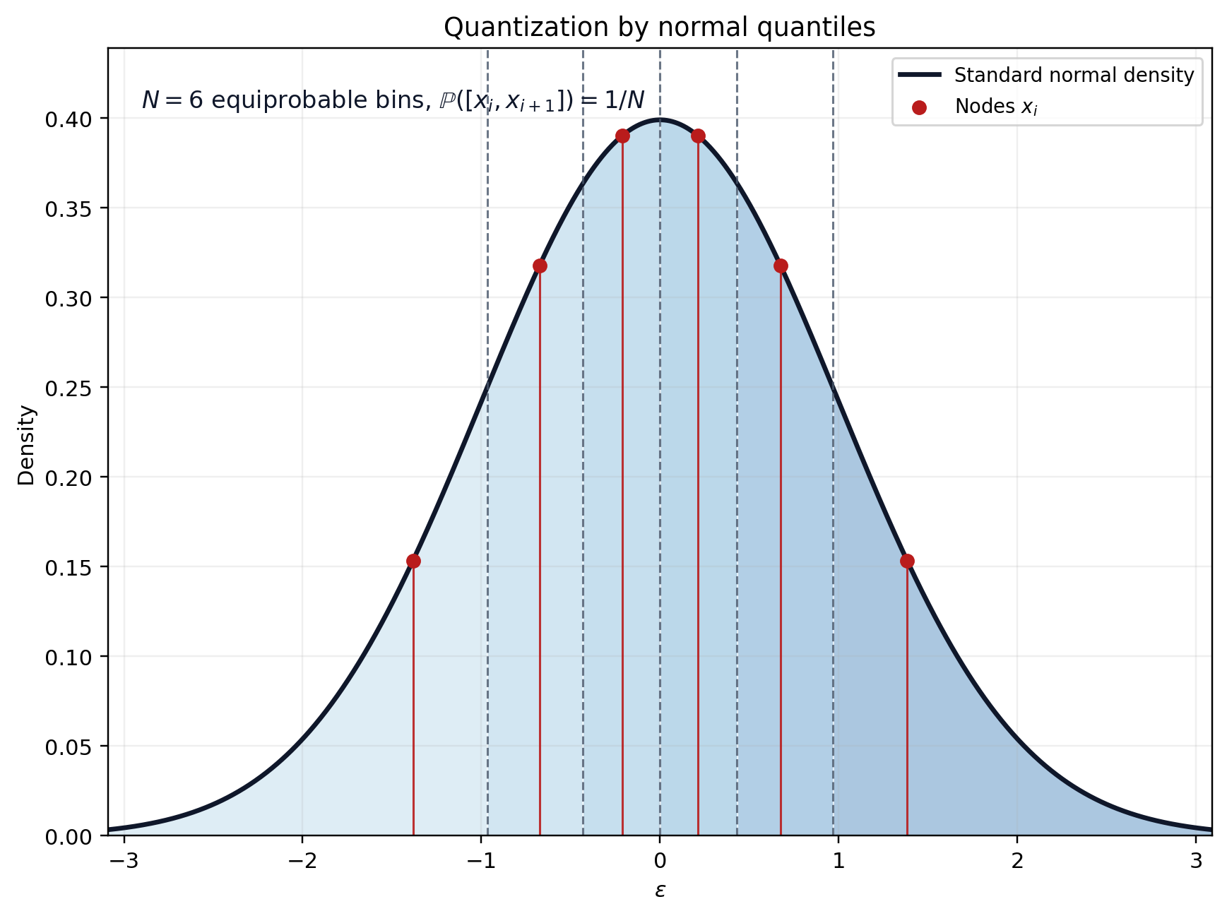
Quantization using quantiles

Equiprobable discretization

  • Works for any distribution with pdf \(\mu\) and cdf \(\mu\)

Split the space into \(N\) equiprobable quantiles: \[(I_i=[a_i,a_{i+1}])_{i=1:N}\] such that \(\mathbb{P}(\epsilon \in I_i)=\frac{1}{N}\)

This yields: \(a_1=-\infty, a_{N+1}=\infty, a_i = \xi^{-1}\left(\frac{i-1}{N}\right)\)

Choose the nodes as the median of each interval: \[\mathbb{P}(\epsilon\in[a_i,x_i]) = \mathbb{P}(\epsilon\in[x_i,a_{i+1}])\] This yields: \(\boxed{x_i = \xi^{-1}\left(\frac{i-0.5}{N}\right)}\)

The quantization is simply \((w_i, x_i)_{i=1:N}\) with \(w_i = 1/N\).
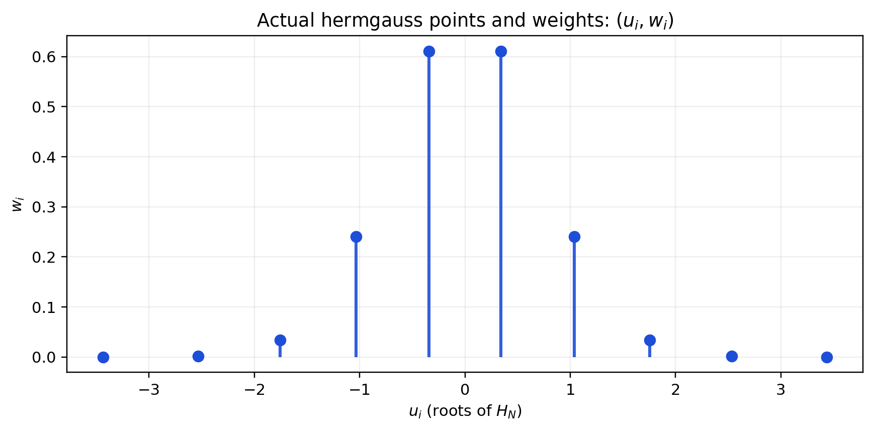
Equiprobable quantization of a normal distribution using quantile bins and median nodes.

Gauss-Hermite

Suppose \(f\in \mathcal{F}\) a Banach space of functions with scalar values., \(\epsilon\) a normal gaussian variable (stdev 1).

Define \(I(f) = E_{\epsilon} f(\epsilon)\).

Take a family of polynomials \(P_n\) orthogonal with respect to the weight function \(\mu(u) = e^{-u^2}\), i.e. such that \[\int_{-\infty}^{\infty} P_n(u) P_m(u) \mu(u) du = 0\] for \(n\neq m\). Suppose these polynomials (hermite polynomials) are dense in \(\mathcal{F}\) (they can approximate any function in \(\mathcal{F}\) with arbitrary precision).

Intuition from linear algebra: \(I\) restricted to \(\mathcal{F}_{N-1}\) is a linear form with \(N\) degrees of freedom. Given any \(N\) points \((\epsilon_n)_{n=1:N}\), we can thus find \(N\) weights \((w_n)_{n=1:N}\) such that \[\left.\left(f\rightarrow\sum_{n=1}^N w_n f(\epsilon_n) \right)\right|_{\mathcal{F}_{N-1}}= \left.I\right|_{\mathcal{F}_{N-1}}\]

  • We have formula that is exact for polynomials of order \(N-1\) or less
  • Will work well if \(f\) can be approximated by polynomials

Gauss quadrature magic (with real nodes and positive weights): there is a unique way to choose \(\epsilon_n\)and \(w_n\) such that \[\left.\left(f\rightarrow\sum_{n=1}^N w_n f(\epsilon_n) \right)\right|_{\mathcal{F}_{2N-1}}= \left.I\right|_{\mathcal{F}_{2N-1}}\]

  • for \(\epsilon_n\): the roots of the \(N\)-th hermite polynomial
  • we need the values of \(f\) at \(N\) points: the formula is exact if \(f\) is a polynomial of order \(2N-1\) or less!

Gauss-Hermite

  • Very accurate if a function can be approximated by polynomials
  • Bad:
    • imprecise if function \(f\) has kinks or non local behaviour
      • points \(\epsilon_n\) can be very far from the origin (see below)
    • not super easy to compute weights and nodes (but there are good libraries)
Gauss-Hermite nodes and effective weights over a standard normal density, showing nodes far in the tails.

Gauss-*

Same logic can be applied to compute integration with weight function \(w(x)\):

\[\int_a^b f(x) w(x)\]

Use polynomials orthogonal with respect to \(w\):

  • Gauss-Hermite:
    • \(w(x) = e^{-x^2}\), \([a,b] = [-\infty, \infty]\)
    • to compute expectations with respect to normal distribution
  • Gauss-Legendre:
    • \(w(x) = 1\)
    • to compute integrals without weight on a bounded interval
  • Gauss-Chebychev:
    • \(w(x)=\sqrt{1-x^2}\), \([a,b] = [-1, 1]\)
    • for periodic functions

In practice

Beware that gauss-hermite weight are given for the normalized gaussian+ law:

\[\frac{1}{\sqrt{2 \pi \sigma^2}}\int f(x) e^{-\frac{x^2}{2\sigma^2}}dx = {\frac{1}{\sqrt{\pi}}}\int f(u {\sigma \sqrt{2}}) e^{-{u^2}}du \]

Compute

\[\mathbb{E}_{\epsilon}[f(\epsilon)] \approx {\frac{1}{\sqrt{\pi}}}\sum_n w_n f(\epsilon_n {\sigma \sqrt{2}})\]

using FastGaussQuadrature

x, w = gausshermite( 10 );
x = x.*σ*sqrt(2) # renormalize nodes
s = sum( w_*X(exp(x_)) for (w_,x_) in zip(w,x))
s /= sqrt(\pi) # renormalize output

Discretizing an AR1

Discretizing an AR1

  • Take \(AR1\) process \[x_t = \rho x_{t-1} + \epsilon_t\]
    • with \(|\rho| <1\) and \(\epsilon \sim N(0,\sigma)\)
  • Can we replace \((x_t)\) by a discrete markov chain?
    • with finite number of states \(N\) and transition matrix \(\P\) of size \(N\times N\).
    • approximate version:
      • good time \(x^g\) and bad time \(x^b\). Probability \(\pi\) of staying in the same, \(1-\pi\) of switching.
    • two systematic methods (available in QuantEcon.jl)
      • Tauchen
      • Rouwenhorst

AR1: Tauchen

Reminder: The unconditional distribution of an AR1 is a normal law \(\mathcal{N}(0,\frac{\sigma}{\sqrt{1-\rho^2}})\)

Algorithm:

  • Choose \(m>0\), typically \(m=3\)
  • Bound the process: \(\underline{x} = -m \frac{\sigma}{\sqrt{1-\rho^2}}\) and \(\overline{x} = m \frac{\sigma}{\sqrt{1-\rho^2}}\)
  • Define the \(N\) discretized points (\(i\in[1,n]\)): \(y_i = \underline{x} + \frac{i-1}{N-1}(\overline{x}-\underline{x})\)
  • Define the transitions:

\[\begin{eqnarray} \pi_{ij} & = & \mathbb{P} \left( y_{t+1}=y_j|y_t=y_i\right)\\ & = & \mathbb{P} \left( |y_{t+1}-y_j| = \inf_k |y_{t+1}-y_k| \left| y_t=y_i \right. \right) \end{eqnarray}\]

AR1: Tauchen (2)

  • Formulas \(\delta=\frac{\overline{x}-\underline{x}}{N-1}\), \(F\) the cdf of \(\mathcal{N}(0,\sigma^2)\), and \(\pi_{ij}\) the transition matrix:

    • if \(1<j<N\)

      \[\pi_{ij} = F\left(\frac{y_j + \delta/2-\rho y_i}{\sigma_{\epsilon}}\right) - F\left(\frac{y_j - \delta/2-\rho y_i}{\sigma_{\epsilon}}\right)\]

    • if \(j=1\)

      \[\pi_{i1} = F\left(\frac{y_1 + \delta/2-\rho y_i}{\sigma_{\epsilon}}\right)\]

    • if \(j=N\)

      \[\pi_{iN} = 1- F\left(\frac{y_N - \delta/2-\rho y_i}{\sigma_{\epsilon}}\right)\]

How to assess the quality of approximation ?

  • compare generated stationary moments between discretized process and true AR1:

    • E(), Var(), ACor()
  • by looking at the exact ergodic distribution or by doing some simulations

  • not very precise when then process is very persistent \(\rho\approx 1\)

Rouvenhorst method (1)

  • N = 2
    • choose \(y_1=-\psi\), \(y_2=\psi\)
    • define transition matrix: \[\Theta_2 = \begin{bmatrix} p & 1-p\\\\ 1-q & q \end{bmatrix}\]
    • choose \(p\), \(q\) and \(\psi\) to match some moments: \(E()\), \(Var()\), \(ACor()\)
      • they can be computed analytically for AR1 and for discretized version.

Rouvenhorst method (2)

  • N >2 \[\Theta_N = p \begin{bmatrix} \Theta_{N-1} & 0\\\\ 0 & 0 \end{bmatrix} + (1-p) \begin{bmatrix} 0 & \Theta_{N-1} \\\\ 0 & 0 \end{bmatrix} + (1-q) \begin{bmatrix} 0 & 0\\\\ \Theta_{N-1} & 0 \end{bmatrix} + q \begin{bmatrix} 0 & 0\\\\ 0 & \Theta_{N-1} \end{bmatrix} \]
  • Normalize all lines

Rouvenhorst method (3)

  • Procedure converges to Bernouilli distribution.

  • Moments can be computed in closed form:

    • \(E() = \frac{(q-p)\psi}{2-(p+q)}\)
    • \(Var() = \psi^2 \left[ 1-4 s (1-s) + \frac{4s(1-s)}{N-1}\right]\)
    • \(Acor()= p+q-1\)
  • Rouwenhorst method performs better for highly correlated processes