Introduction to Machine Learning
Data-Based Economics, ESCP, 2025-2026
2026-02-04
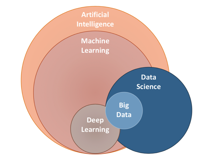
What about artificial intelligence ?
- AIs
- think and learn
- mimmic human cognition
Tabular Data
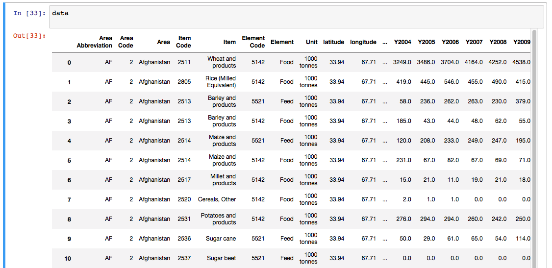
tabular data
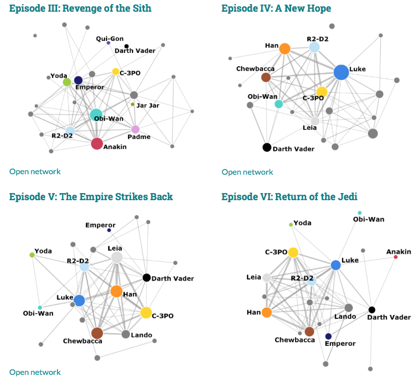
Networks
- Banking networks
- Production network
Big Subfields of Machine Learning
- Traditional classification
- supervised (labelled data)
- regression: predict quantity
- classification: predict index (categorical variable)
- unsupervised (no labels)
- dimension reduction
- clustering
- semi-supervised / self-supervised
- reinforcement learning
- supervised (labelled data)
- Bazillions of different algorithms: https://scikit-learn.org/stable/user_guide.html
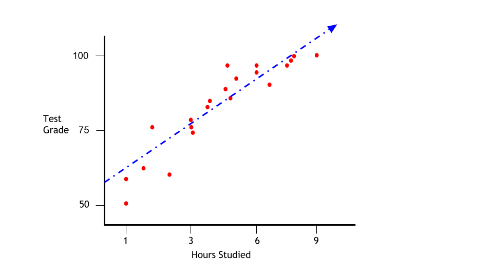
supervised: regression:
| Age | Activity | Salary |
|---|---|---|
| 23 | Explorer | 1200 |
| 40 | Mortician | 2000 |
| 45 | Mortician | 2500 |
| 33 | Movie Star | 3000 |
| 35 | Explorer | ??? |
supervised: regression:
- Predict: \(y = f(x; \theta)\)
| Age | Salary | Activity |
|---|---|---|
| 23 | 1200 | Explorer |
| 40 | 2000 | Mortician |
| 45 | 2500 | Mortician |
| 33 | 3000 | Movie Star |
| 35 | 3000 | ??? |
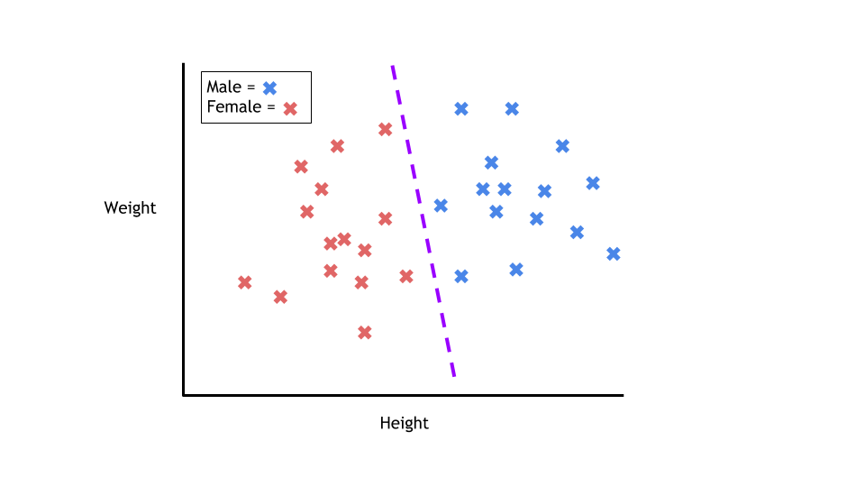
supervised: classification
- Output is discrete
- A regression with discrete output
- train \(\sigma(f(x; \theta))\) where \(\sigma(x)=\frac{1}{1-e^{-x}}\)
| Age | Salary | Activity |
|---|---|---|
| 23 | 1200 | Explorer |
| 40 | 2000 | Mortician |
| 45 | 2500 | Mortician |
| 33 | 3000 | Movie Star |
| 35 | 3000 | ??? |
unsupervised
| Age | Salary | Activity |
|---|---|---|
| 23 | 1200 | Explorer |
| 40 | 2000 | Mortician |
| 45 | 2500 | Mortician |
| 33 | 3000 | Movie Star |
| 35 | 3000 | Explorer |
unsupervised
- organize data without labels
- dimension reduction: describe data with less parameters
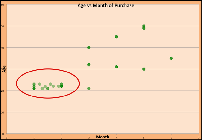
- clustering: sort data into “similar groups” (exemple)
unsupervised: clustering
unsupervised: clustering
Women buying dresses during the year:
Long data
Long data is characterized by a high number of observations.
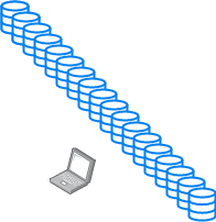
- Modern society is gathering a lot of data.
- in doesn’t fit in the computer memory so we can’t run a basic regression
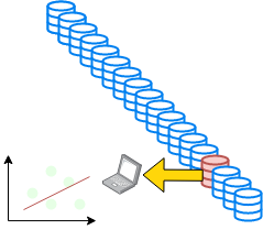
- In some cases we would also like to update our model continuously:
- incremental regression
We need a way to fit a model on a subset of the data at a time.
Training: Gradient Descent
How do we minimize a function \(f(a,b)\)?
Gradient descent:
- \(a_k, b_k\) given
- compute the gradient (slope) \(\nabla_{a,b} f = \begin{bmatrix} \frac{\partial f}{\partial a} \\\\ \frac{\partial f}{\partial b}\end{bmatrix}\)
- follow the steepest slope: (Newton Algorithm)
- \[ \begin{bmatrix} a_{k+1} \\\\ b_{k+1} \end{bmatrix} \leftarrow \begin{bmatrix} a_k \\\\ b_k \end{bmatrix} - \nabla_{a,b} f\]
- but not too fast: use learning rate \(\lambda\): \[ \begin{bmatrix} a_{k+1} \\\\ b_{k+1} \end{bmatrix} \leftarrow (1-\lambda) \begin{bmatrix} a_k \\\\ b_k \end{bmatrix} + \lambda (- \nabla_{a,b} f )\]
Some possible issues
- In practice, choosing the right learning rate \(\lambda\) is crucial
- \(\lambda\) is a metaparameter of the model training.
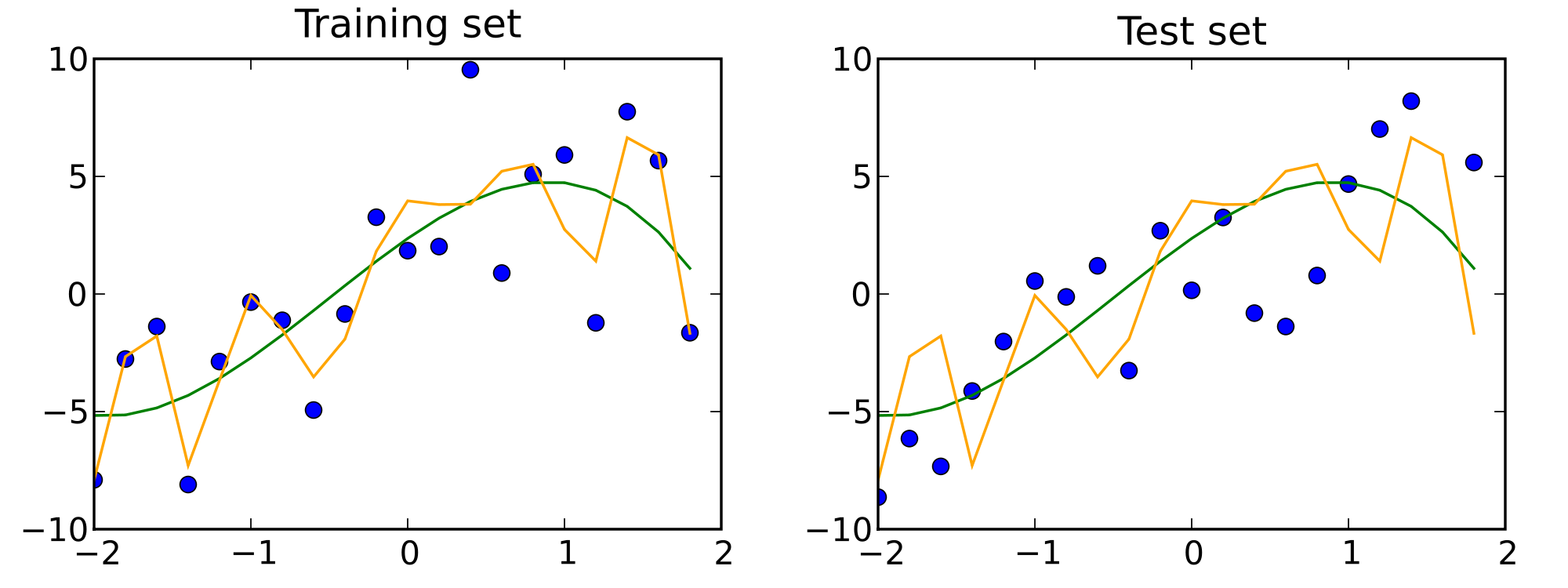
Traintest
The test set reveals that orange model is overfitting.
How to choose the validation set?
A more robust solution: \(k\)-fold validation
- split dataset randomly in \(K\) subsets of equal size \(S_1, ... S_K\)
- use subset \(S_i\) as test set, the rest as training set, compute the score
- compare the scores obtained for all \(i\in[1,K]\)
- they should be similar (compute standard deviation)
- average them