Linear Regression

Data-Based Economics, ESCP, 2025-2026

Pablo Winant

2026-01-21

Table of contents

• Descriptive Statistics
• Fitting the data
• Explained Variance
• Statistical inference
• Fact Check

Descriptive Statistics

A Simple Dataset

Duncan’s Occupational Prestige Data

• Many occupations in 1950.

• Education and prestige associated to each occupation

• \(x\): education

  • Percentage of occupational incumbents in 1950 who were high school graduates

• \(y\): income

  • Percentage of occupational incumbents in the 1950 US Census who earned $3,500 or more per year

• \(z\): Percentage of respondents in a social survey who rated the occupation as “good” or better in prestige

Quick look

Import the data from statsmodels’ dataset:

import statsmodels.api as sm
dataset = sm.datasets.get_rdataset("Duncan", "carData")
df = dataset.data
df.head()

	type	income	education	prestige
rownames
accountant	prof	62	86	82
pilot	prof	72	76	83
architect	prof	75	92	90
author	prof	55	90	76
chemist	prof	64	86	90

Descriptive Statistics

For any variable \(v\) with \(N\) observations:

• mean: \(\overline{v} = \frac{1}{N} \sum_{i=1}^N v_i\)
• variance \(V({v}) = \frac{1}{N} \sum_{i=1}^N \left(v_i - \overline{v} \right)^2\)
• standard deviation : \(\sigma(v)=\sqrt{V(v)}\)

df.describe()

	income	education	prestige
count	45.000000	45.000000	45.000000
mean	41.866667	52.555556	47.688889
std	24.435072	29.760831	31.510332
min	7.000000	7.000000	3.000000
25%	21.000000	26.000000	16.000000
50%	42.000000	45.000000	41.000000
75%	64.000000	84.000000	81.000000
max	81.000000	100.000000	97.000000

Relation between variables

• How do we measure relations between two variables (with \(N\) observations)
  • Covariance: \(Cov(x,y) = \frac{1}{N}\sum_i (x_i-\overline{x})(y_i-\overline{y})\)
  • Correlation: \(Cor(x,y) = \frac{Cov(x,y)}{\sigma(x)\sigma(y)}\)
• By construction, \(Cor(x,y)\in[-1,1]\)
  • if \(Cor(x,y)>0\), x and y are positively correlated
  • if \(Cor(x,y)<0\), x and y are negatively correlated
• Interpretation:
  • no interpretation!
  • correlation is not causality
  • also: data can be correlated by pure chance (spurious correlation)

Examples

df[['income','education','prestige']].cov()

	income	education	prestige
income	597.072727	526.871212	645.071212
education	526.871212	885.707071	798.904040
prestige	645.071212	798.904040	992.901010

df[['income','education','prestige']].corr()

	income	education	prestige
income	1.000000	0.724512	0.837801
education	0.724512	1.000000	0.851916
prestige	0.837801	0.851916	1.000000

Can we visualize correlations?

Quick

from matplotlib import pyplot as plt
plt.plot(df['education'],df['income'],'o')
plt.grid()
plt.xlabel("Education")
plt.ylabel("Income")
plt.savefig("data_description.png")

from matplotlib import pyplot as plt
plt.plot(df['education'],df['prestige'],'o')
plt.grid()
plt.xlabel("Education")
plt.ylabel("Prestige")
plt.savefig("data_description.png")

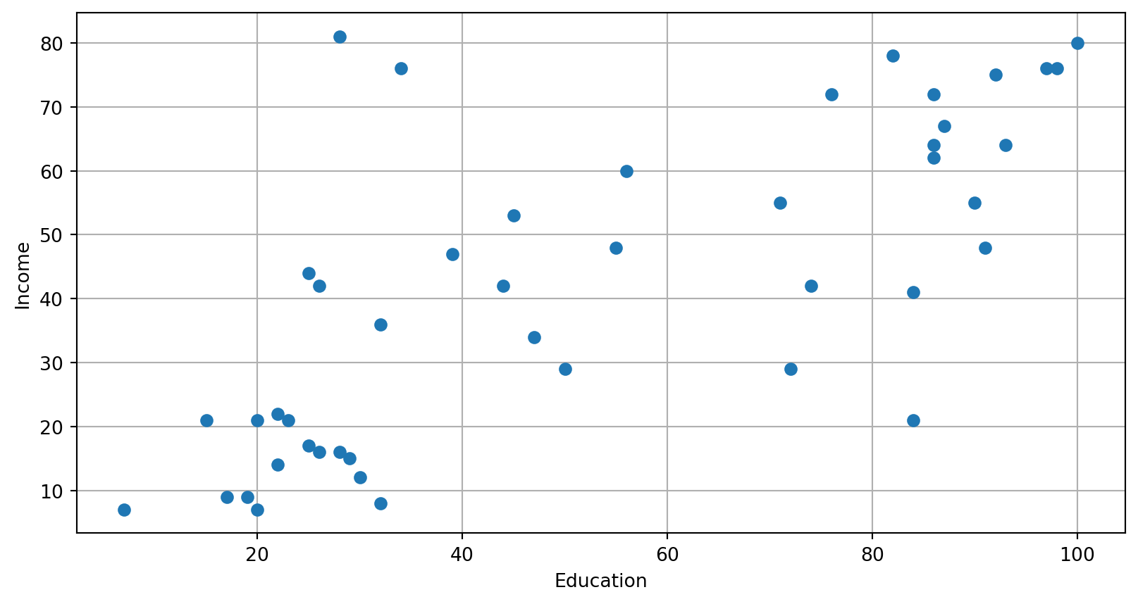
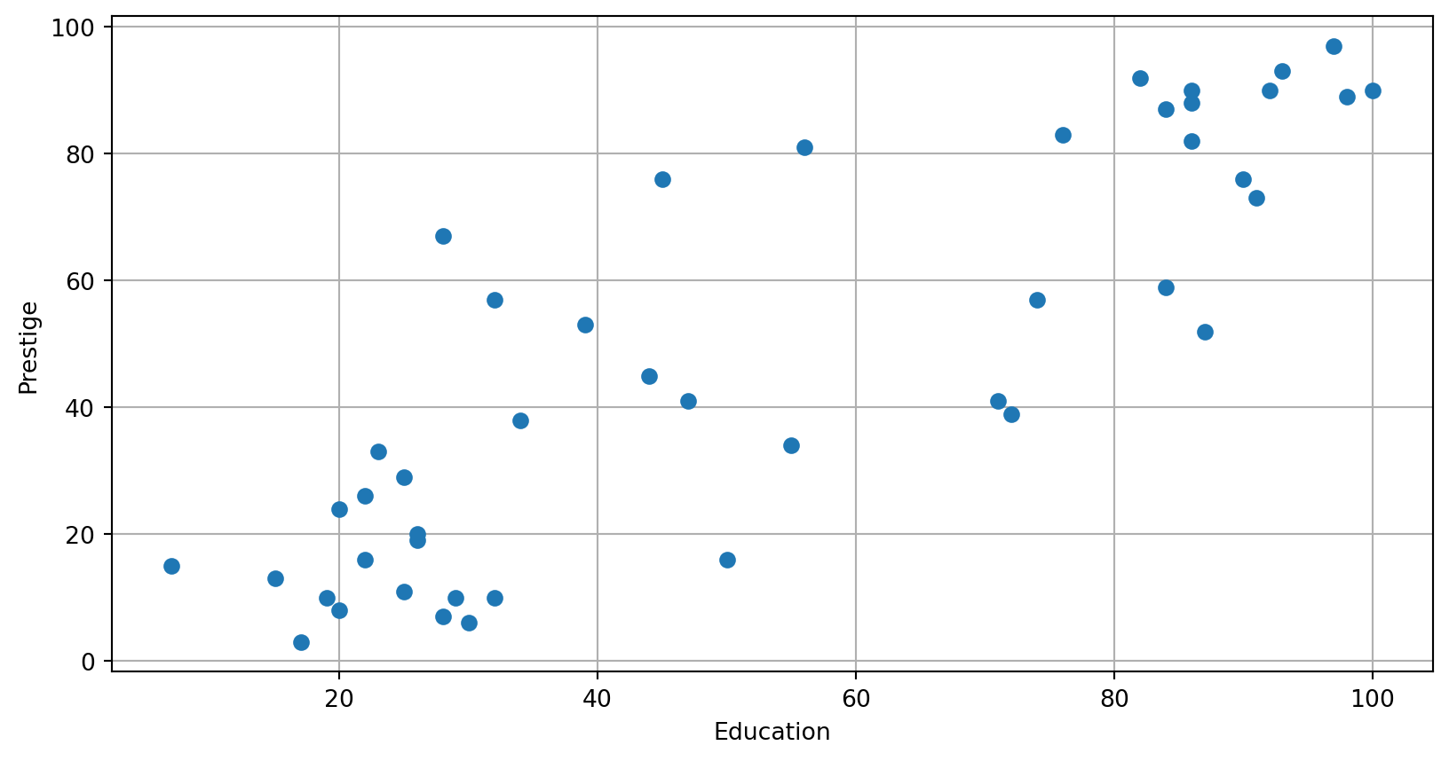
Quick look

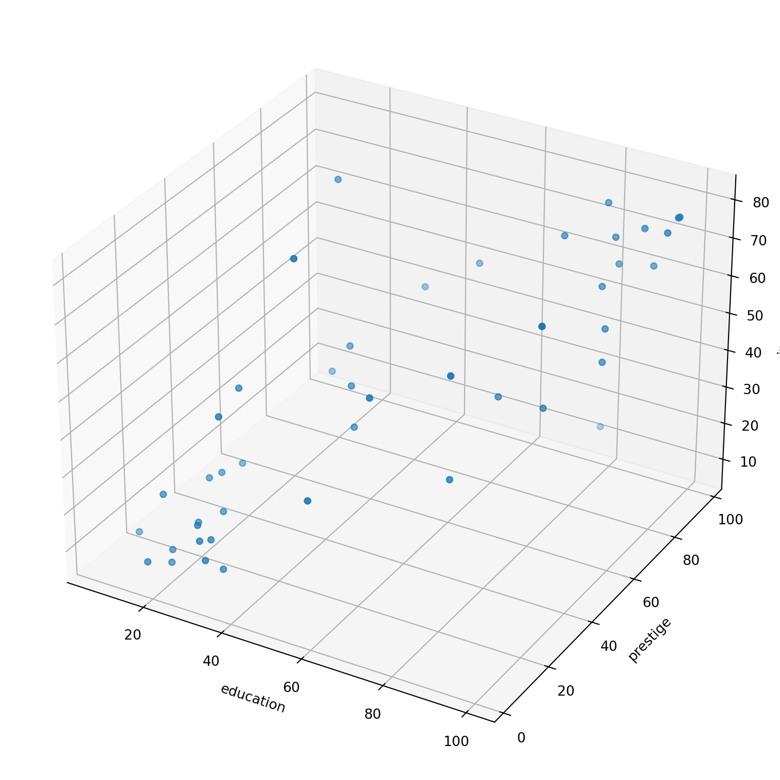
Using matplotlib (3d)

Quick look

import seaborn as sns
sns.pairplot(df[['education', 'prestige', 'income']])

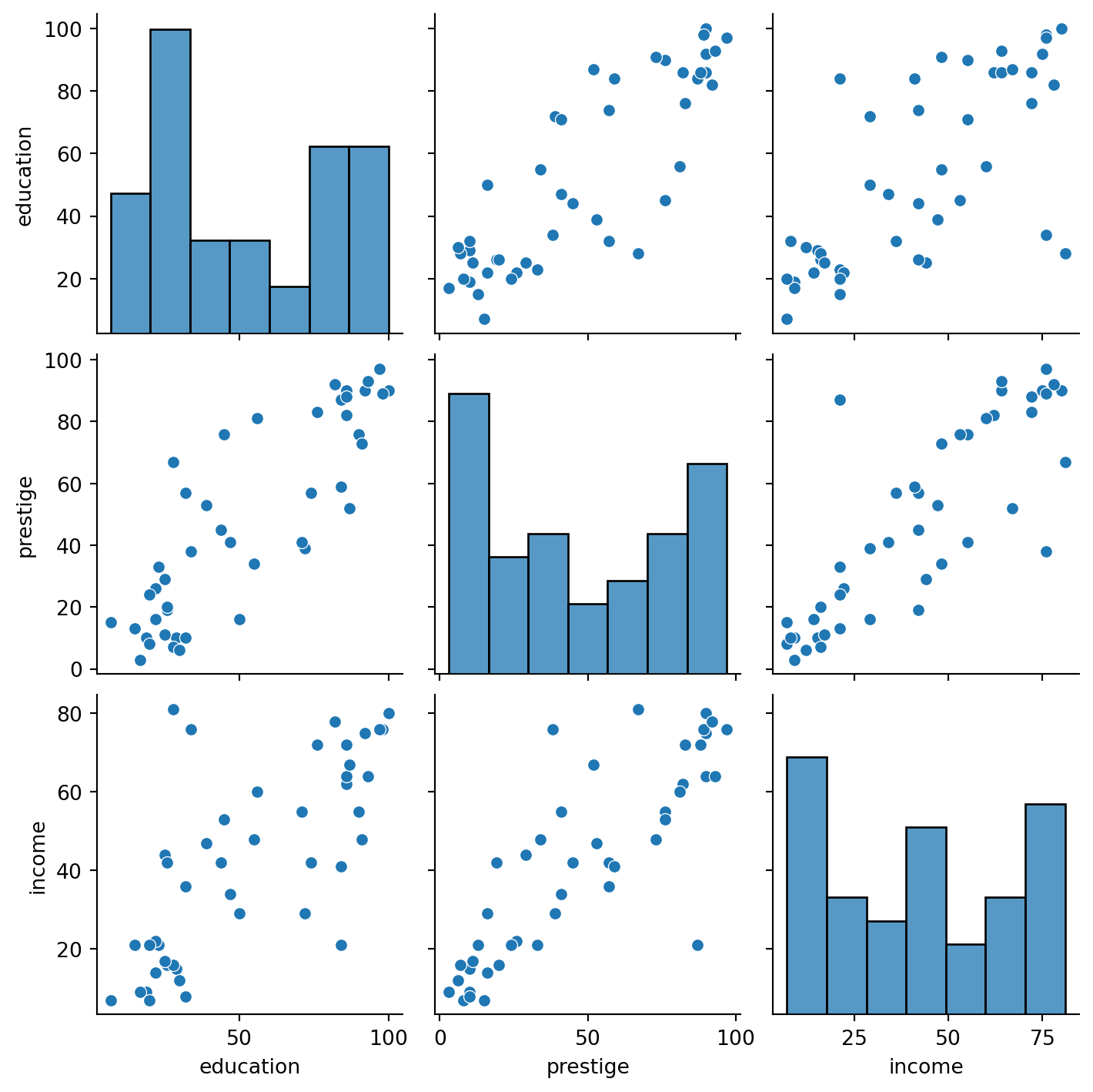
The pairplot made with seaborn gives a simple sense of correlations as well as information about the distribution of each variable.

Fitting the data

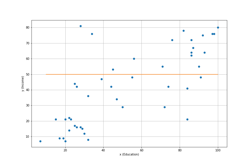
A Linear Model

Now we want to build a model to represent the data:

Consider the line: \[y = α + β x\]

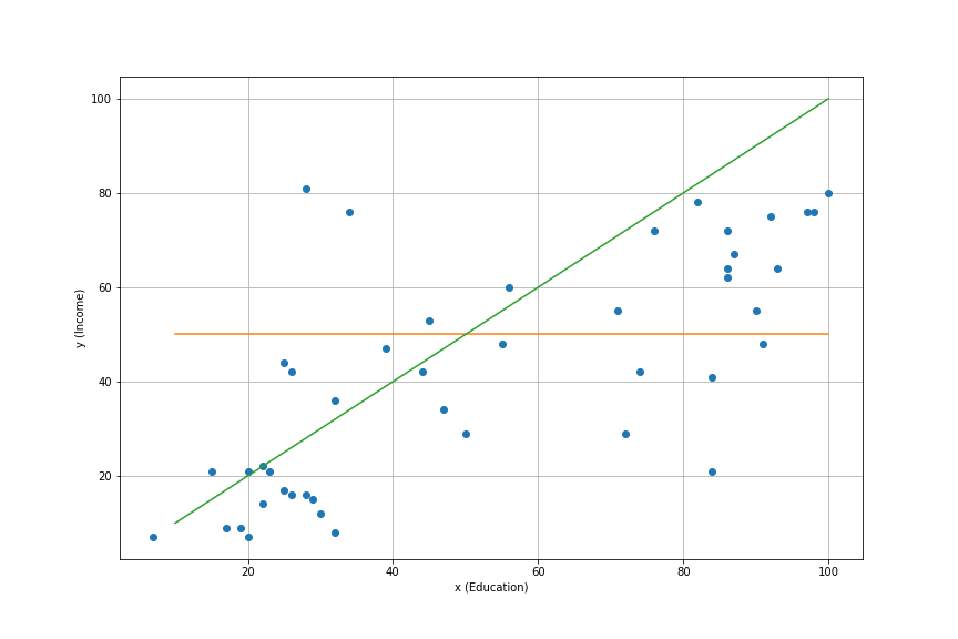
Several possibilities. Which one do we choose to represent the model?

We need some criterium.

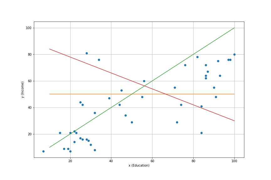
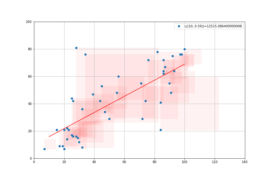
Least Square Criterium

• Compare the model to the data: \[y_i = \alpha + \beta x_i + \underbrace{e_i}_{\text{prediction error}}\]
• Square Errors \[{e_i}^2 = (y_i-\alpha-\beta x_i)^2\]
• Loss Function: sum of squares \[L(\alpha,\beta) = \sum_{i=1}^N (e_i)^2\]

Minimizing Least Squares

• Try to chose \(\alpha, \beta\) so as to minimize the sum of the squares \(L(α, β)\)
• It is a convex minimization problem: unique solution
• This direct iterative procedure is used in machine learning

Ordinary Least Squares (1)

• The mathematical problem \(\min_{\alpha,\beta} L(\alpha,\beta)\) has one unique solution¹

• Solution is given by the explicit formula: \[\hat{\alpha} = \overline{y} - \hat{\beta} \overline{x}\] \[\hat{\beta} = \frac{Cov({x,y})}{Var(x)} = Cor(x,y) \frac{\sigma(y)}{\sigma({x})}\]

• \(\hat{\alpha}\) and \(\hat{\beta}\) are estimators.

  • Hence the hats.
  • More on that later.

1. Proof not important here.

Concrete Example

In our example we get the result: \[\underbrace{y}_{\text{income}} = 10 + 0.59 \underbrace{x}_{education}\]

We can say:

• income and education are positively correlated
• a unit increase in education is associated with a 0.59 increase in income
• a unit increase in education explains a 0.59 increase in income

But:

• here explains does not mean cause

Explained Variance

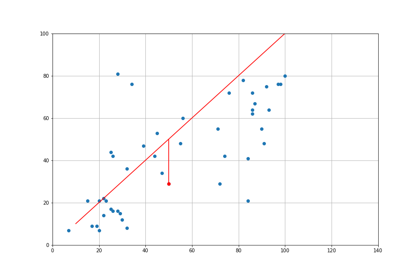
Predictions

It is possible to make predictions with the model:

• How much would an occupation which hires 60% high schoolers fare salary-wise?

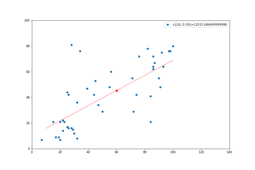
• Prediction: salary measure is \(45.4\)

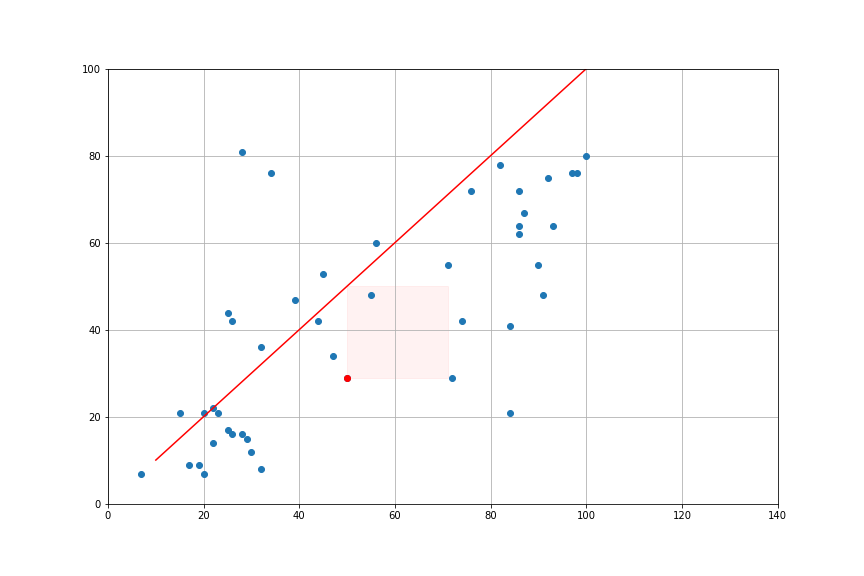
OK, but that seems noisy, how much do I really predict ? Can I get a sense of the precision of my prediction ?

Look at the residuals

• Plot the residuals:

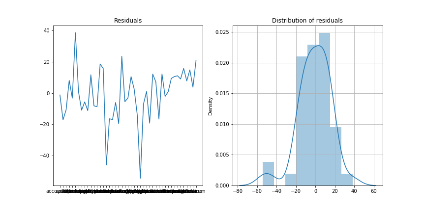
• Any abnormal observation?
• Theory requires residuals to be:
  • zero-mean
  • non-correlated
  • normally distributed
• That looks like a normal distribution
  • standard deviation is \(\sigma(e_i) = 16.84\)
• A more honnest prediction would be \(45.6 ± 16.84\)

What could go wrong?

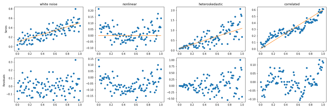
• a well specified model, residuals must look like white noise (i.i.d.: independent and identically distributed)
• when residuals are clearly abnormal, the model must be changed

Explained Variance

• What is the share of the total variance explained by the variance of my prediction? \[R^2 = \frac{\overbrace{Var(\hat{\alpha} + \hat{\beta} x_i)}^{ \text{MSS} } } {\underbrace{Var(y_i)}_{ \text{TSS} } } = \frac{MSS}{TSS} = (Cor(x,y))^2\] \[R^2 = 1-\frac{\overbrace{Var(y_i - \hat{\alpha} + \hat{\beta} x_i)}^{\text{RSS}} } { \underbrace{Var(y_i)}_{ {\text{TSS} }}} = 1 - \frac{RSS}{TSS} \]

• MSS: model sum of squares, explained variance
• RSS: residual sum of square, unexplained variance
• TSS: total sum of squares, total variance

• Coefficient of determination is a measure of the explanatory power of a regression
  • but not of the significance of a coefficient
  • we’ll get back to it when we see multivariate regressions
• In one-dimensional case, it is possible to have small R2, yet a very precise regression coefficient.

Graphical Representation

Statistical inference

Statistical model

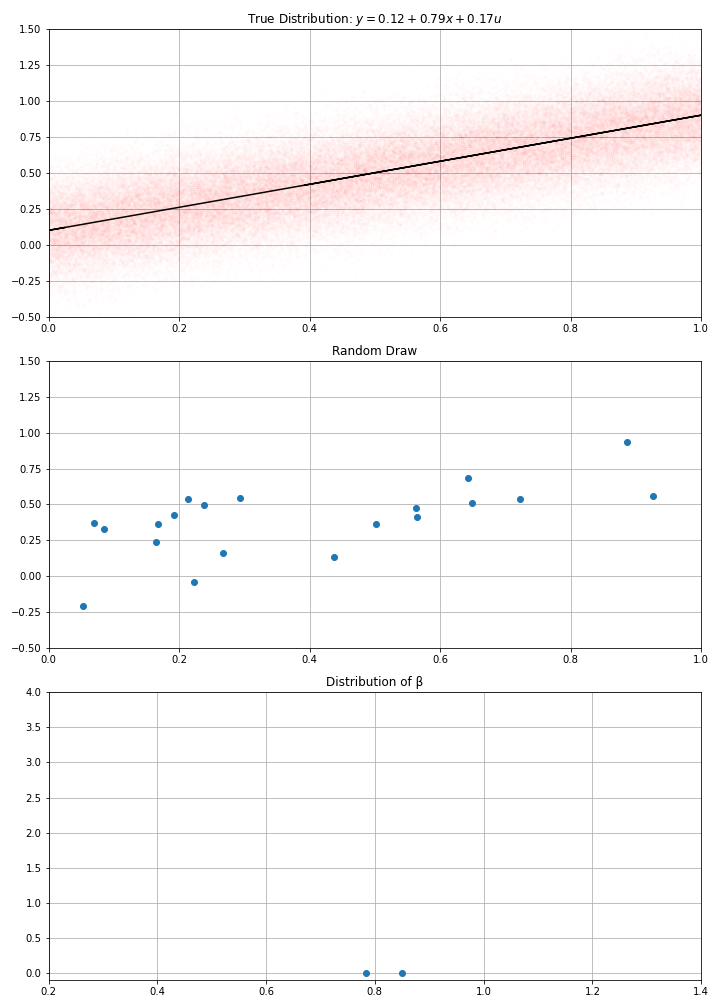
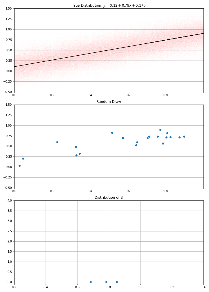
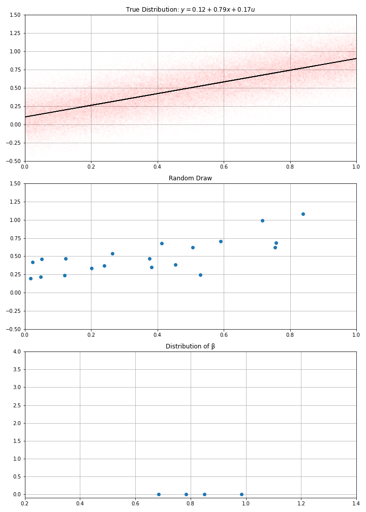
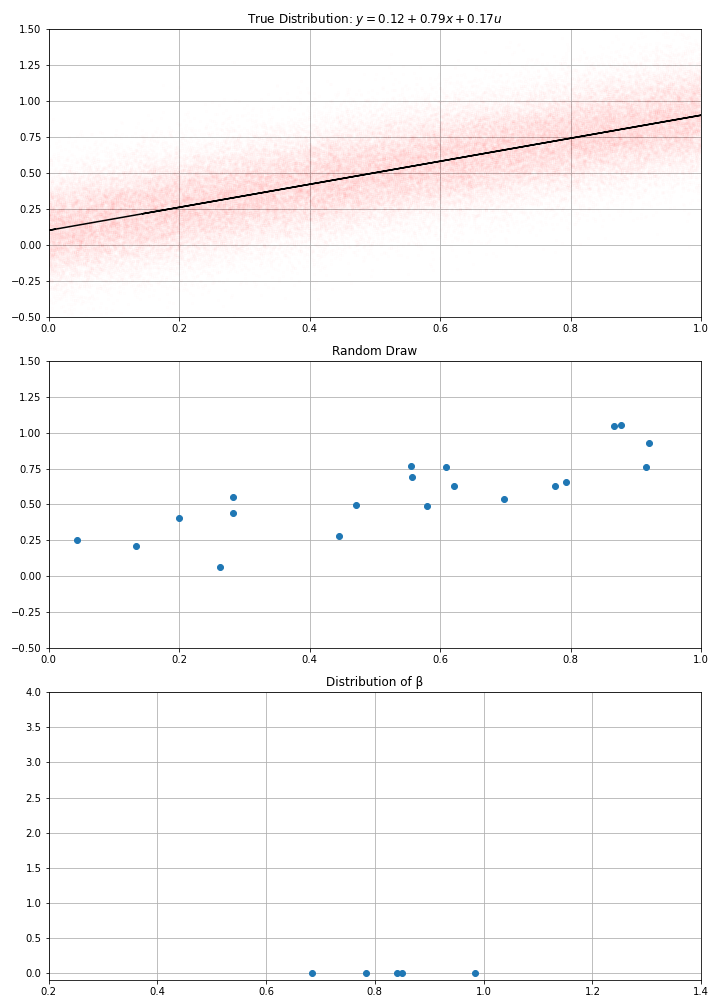
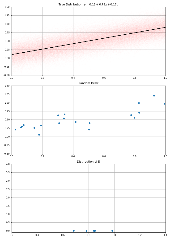
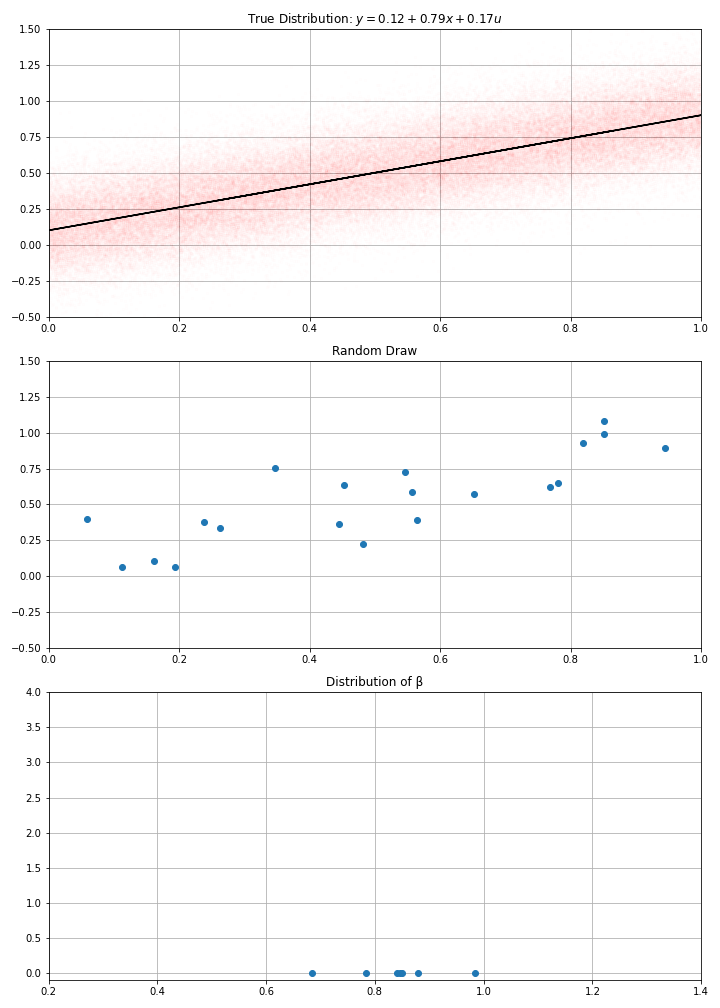
Imagine the true model is: \[y = α + β x + \epsilon\] \[\epsilon_i \sim \mathcal{N}\left({0,\sigma^{2}}\right)\]

• errors are independent …
• and normallly distributed …
• with constant variance (homoscedastic)

Using this data-generation process, I have drawn randomly \(N\) data points (a.k.a. gathered the data)

• maybe an acual sample (for instance \(N\) patients)
• an abstract sample otherwise

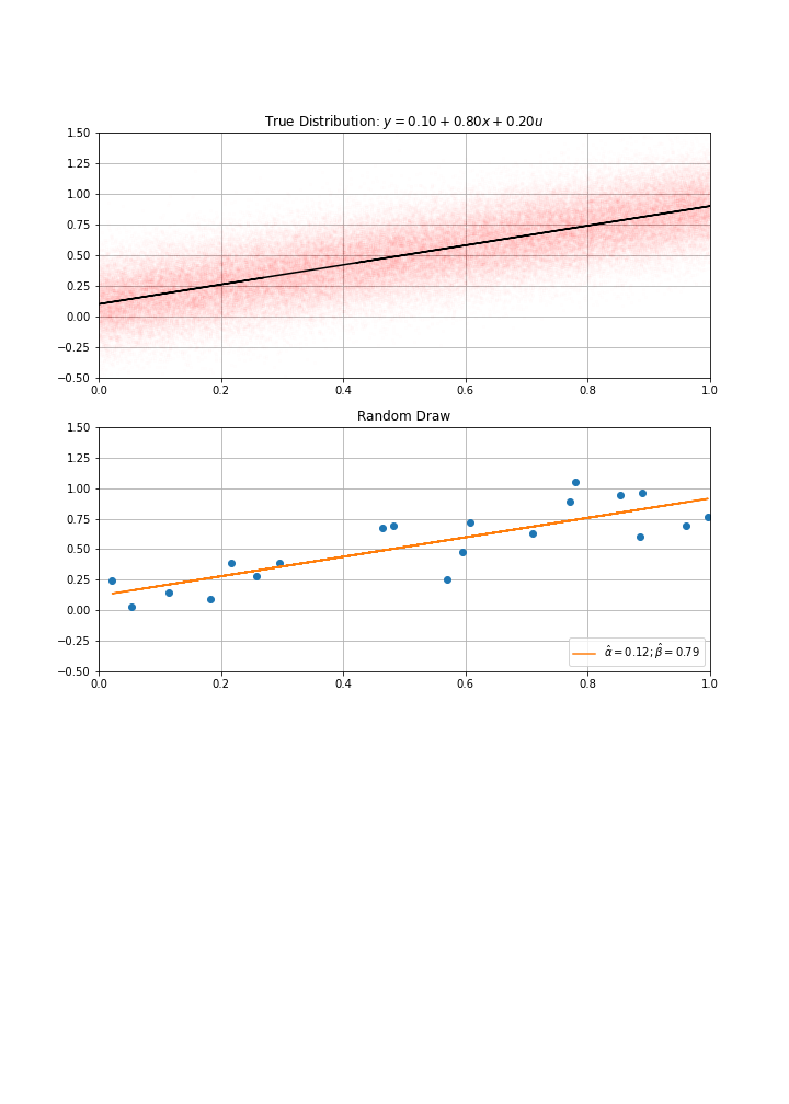
Then computed my estimate \(\hat{α}\), \(\hat{β}\)

How confident am I in these estimates ?

• I could have gotten a completely different one…
• clearly, the bigger \(N\), the more confident I am…

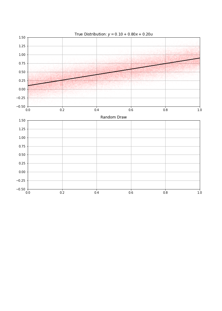
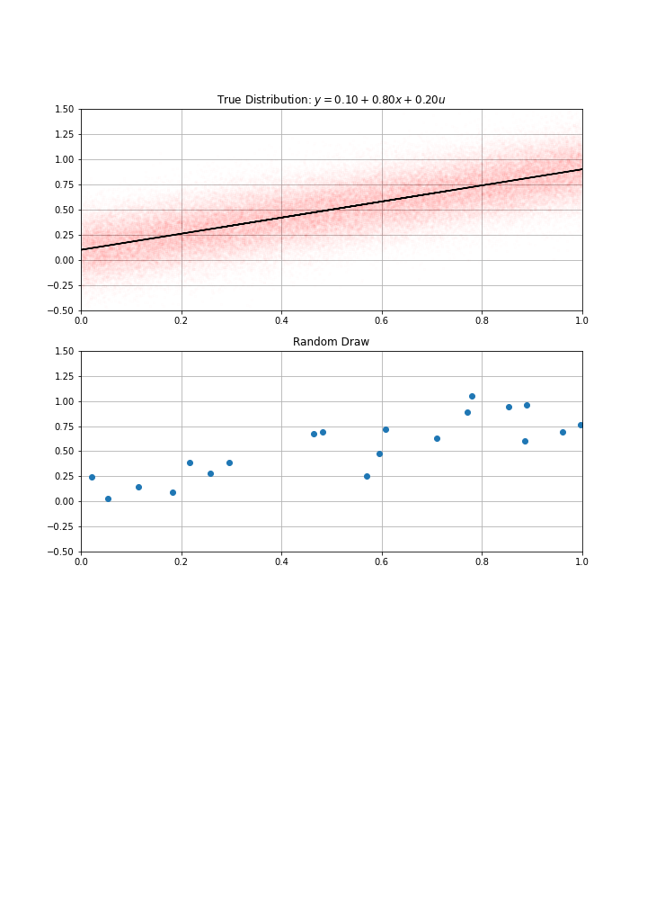
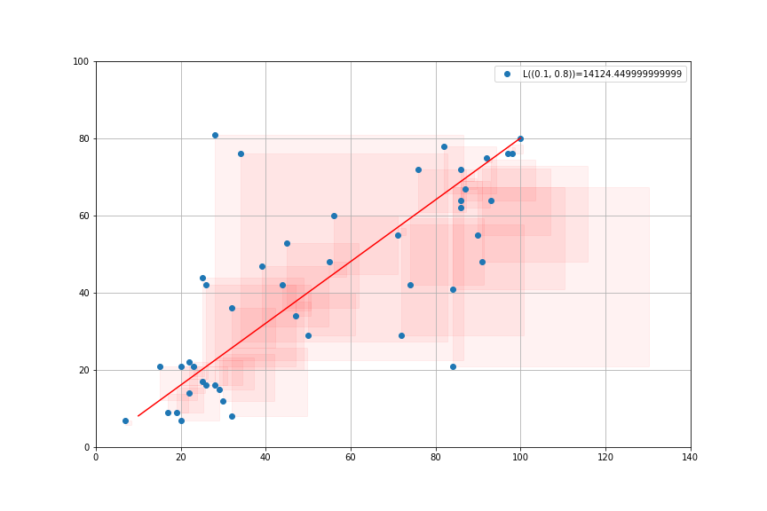
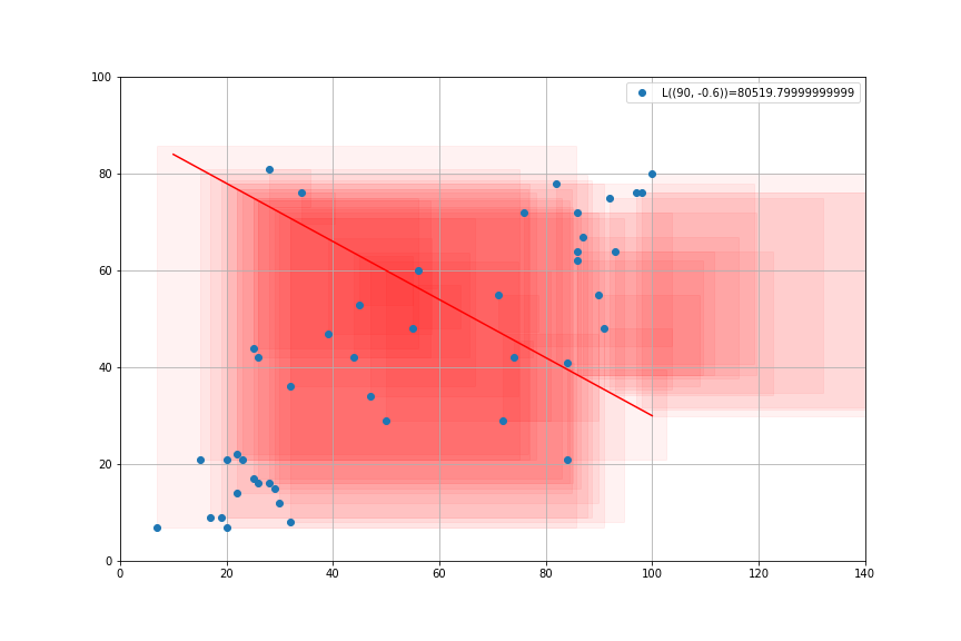
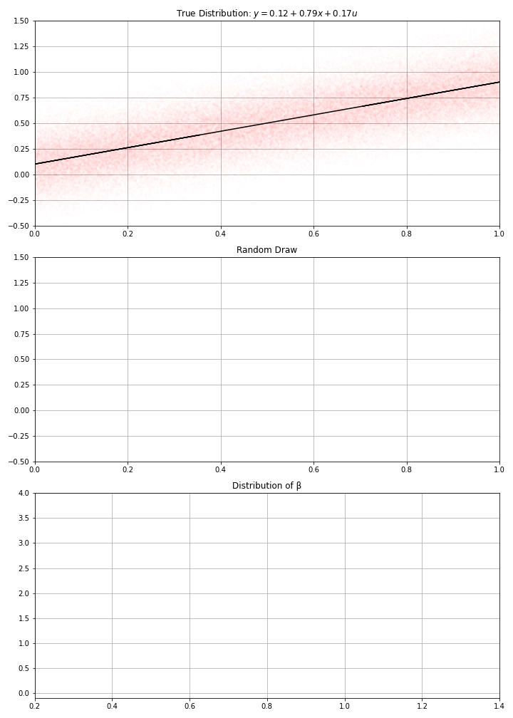
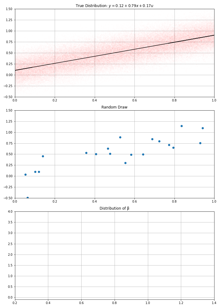
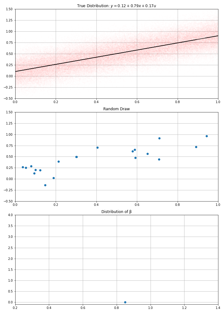
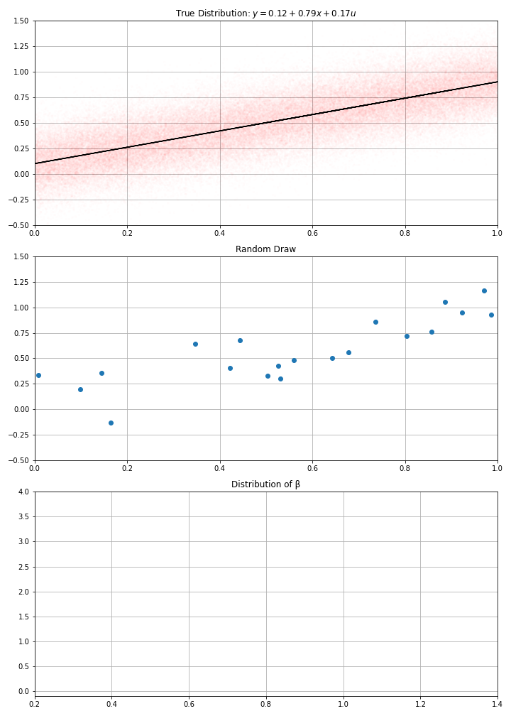
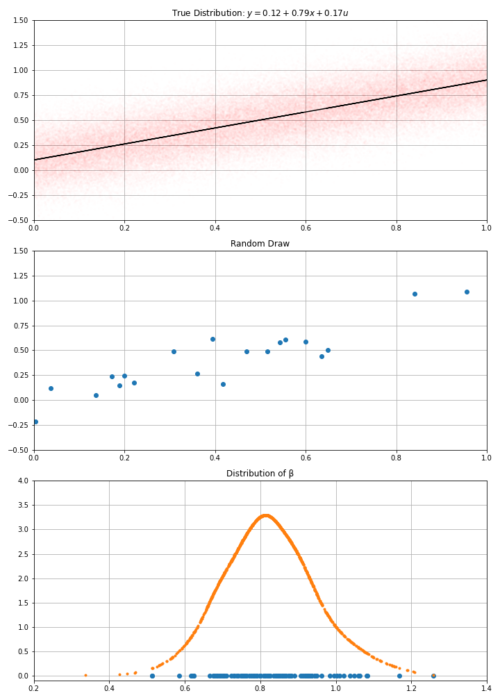
Statistical inference (2)

• Assume we have computed \(\hat{\alpha}\), \(\hat{\beta}\) from the data. Let’s make a thought experiment instead.
• Imagine the actual data generating process was given by \(\hat{α} + \hat{\beta} x + \epsilon\) where \(\epsilon \sim \mathcal{N}(0,Var({e_i}))\)

• If I draw randomly \(N\) points using this D.G.P. I get new estimates.
• And if I make randomly many draws, I get a distribution for my estimate.
  • I get an estimated \(\hat{\sigma}(\hat{\beta})\)
  • were my initial estimates very likely ?
  • or could they have taken any value with another draw from the data ?
  • in the example, we see that estimates around of 0.7 or 0.9, would be compatible with the data
• How do we formalize these ideas?
  • Statistical tests.

First estimates

• Given the true model, all estimators are random variables of the data generating process

• Given the values \(\alpha\), \(\beta\), \(\sigma\) of the true model, we can model the distribution of the estimates.

• Some closed forms:

  • \(\hat{\sigma}^2 = Var(y_i - \alpha -\beta x_i)\) estimated variance of the residuals
  • \(mean(\hat{\beta}) = \beta\) (unbiased)
  • \(\sigma(\hat{\beta}) = \frac{\sigma^2}{Var(x_i)}\)

• These statististics or any function of them can be computed exactly, given the data.

• Their distribution depends, on the data-generating process

• Can we produce statistics whose distribution is known given mild assumptions on the data-generating process?

  • if so, we can assess how likely are our observations

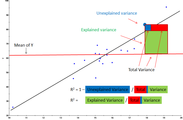
Fisher-Statistic

Test

• Hypothesis H0:
  • \(α=β=0\)
  • model explains nothing, i.e. \(R^2=0\)
• Hypothesis H1: (model explains something)
  • model explains something, i.e. \(R^2>0\)

Fisher Statistics: \[\boxed{F=\frac{Explained Variance}{Unexplained Variance}}\]

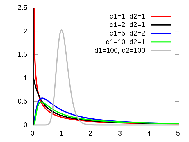
Distribution of \(F\) is known theoretically.

• Assuming the model is actually linear and the shocks normal.
• It depends on the number of degrees of Freedom. (Here \(N-2=18\))
• Not on the actual parameters of the model.

In our case, \(Fstat=40.48\).

What was the probability it was that big, under the \(H0\) hypothesis?

• extremely small: \(Prob(F>Fstat|H0)=5.41e-6\)
• we can reject \(H0\) with \(p-value=5e-6\)

In social science, typical required p-value is 5%.

In practice, we abstract from the precise calculation of the Fisher statistics, and look only at the p-value.

Student test

• So our estimate is \(y = \underbrace{0.121}_{\tilde{\alpha}} + \underbrace{0.794}_{\tilde{\beta}} x\).
  • we know \(\tilde{\beta}\) is a bit random (it’s an estimator): are we even sure \(\tilde{\beta}\) could not have been zero?
• Student Test: H0: \(\beta=0\), H1: \(\beta \neq 0\)
  • Statistics: \(t=\frac{\hat{\beta}}{\sigma(\hat{\beta})}\)
    • intuitively: compare mean of estimator to its standard deviation
    • also a function of degrees of freedom
• Significance levels (read in a table or use software):
  • for 18 degrees of freedom, \(P(|t|>t^{\star})=0.05\) with \(t^{\star}=1.734\)
  • if \(t>t^{\star}\) we are \(95%\) confident the coefficient is significant

Student tables

Confidence intervals

The student test can also be used to construct confidence intervals.

• Given estimate, \(\hat{\beta}\) with standard deviation \(\sigma(\hat{\beta})\)

• Given a probability threshold \(\alpha\) (for instance \(\alpha=0.05\)) we can compute \(t^{\star}\) such that \(P(|t|>t*)=\alpha\)

We construct the confidence interval: \[I^{\alpha} = [\hat{\beta}-t\sigma(\hat{\beta}), \hat{\beta}+t\sigma(\hat{\beta})]\]

Interpretation (⚠: subtle)

• if the true value was outside of the confidence interval, the probability of obtaining the value that we got would be less than 5%
• if we had repeated the experiment many times and computed the confidence interval, the true value would be inside it 95% of the time
• we can say the true value is within the interval with 95% confidence level

Fact Check

Do more firearms reduce homicide?

Claim (common intuition): “More civilian firearms deter crime ⇒ fewer homicides.”

Simple cross-country OLS (26 high-income countries, early 1990s)
\[\text{HomicideRate}_i = \alpha + \beta\,\text{GunAvailability}_i + \varepsilon_i\]

• Gun availability proxied by the Cook index = average of
  (% suicides with a firearm, % homicides with a firearm)

What the bivariate regression finds (Table 2):

• Crude homicide rate: (= 9.2) (p < 0.001), corr = 0.74
  
• Excluding the U.S.: (= 4.9) (p = 0.003), corr = 0.57

Takeaway: The “more guns → less homicide” claim is not supported by this simple cross-country correlation.

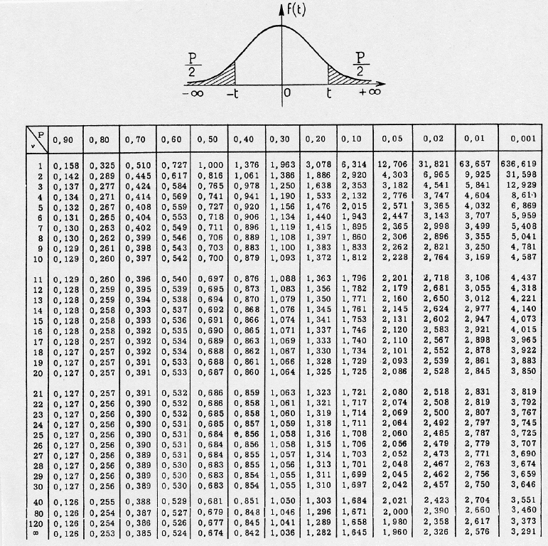
⚠️ Caution (OLS lesson): This is not causal (possible confounding, reverse causality, measurement error). Use it to practice interpreting (), p-values, and thinking about omitted variables.