L’importance des intermédiaires financiers
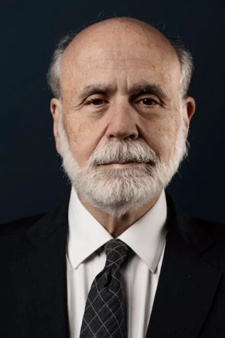
Ben Bernanke
président de la Fed (2006-2014), succédant à Alan Greenspan
surnommé Helicopter Ben
était un spécialiste de la Grande Dépression…
- l’État / la banque centrale auraient dû créer davantage de monnaie
…et a ensuite dû faire face à la Grande Récession
- l’État / la banque centrale auraient dû être plus attentifs à la situation des intermédiaires financiers
a reçu le prix Nobel en 2022 avec Diamond et Dybvig
- pour leurs travaux sur les banques et la nécessité de leur renflouement en période de crise financière
- Bernanke (et d’autres) ont intégré des modèles réalistes de banques (issus de D&D) dans des modèles DSGE
Son discours de réception est en ligne
Marchés du crédit
Les marchés du crédit sont cruciaux pour comprendre :
- les crises financières
- la persistance des récessions “ordinaires”
- la politique monétaire
- la régulation financière et les politiques prudentielles
- désormais intégrées dans la “macropru”, qui occupe une place importante dans les banques centrales
Problèmes liés au crédit
- Information imparfaite et asymétrique
- les emprunteurs connaissent mieux leur capacité financière
- → Aléa moral : peu d’incitations à adopter un comportement assurant le remboursement
- → Problème de sélection adverse
- les emprunteurs les plus risqués ont davantage intérêt à demander des fonds
- Les banques et autres prêteurs traitent ces problèmes avec divers outils :
- relation de longue durée
- filtrage (screening)
- restrictions imposées aux emprunteurs (covenant1)
- suivi (monitoring)
- collatéraux
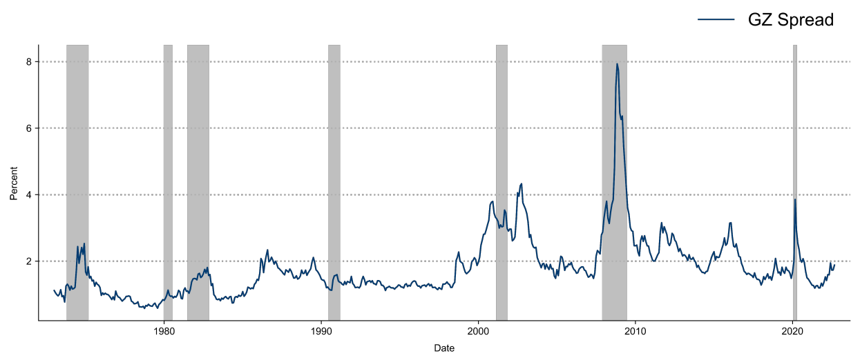
Prime de financement externe
Prime de financement externe
Le coût total d’un prêt pour un emprunteur donné (y compris les coûts liés aux covenants, aux exigences de collatéraux, etc.), moins le taux d’intérêt sans risque (par exemple le rendement des titres publics).
- La prime de financement externe est le coût de l’intermédiation
- c’est une distorsion aux conséquences macroéconomiques
- Elle est différente pour chaque emprunteur
- elle dépend de la taille et du risque
Un enseignement clé de la littérature sur l’intermédiation financière
- La PFE est déterminée par la valeur nette de l’emprunteur et du prêteur
Accélérateur financier1 :
- une PFE plus élevée : crédit plus strict, moins de prêts, ralentissement de l’économie
- une économie affaiblie dégrade la santé financière des prêteurs et des emprunteurs, ce qui augmente la PFE
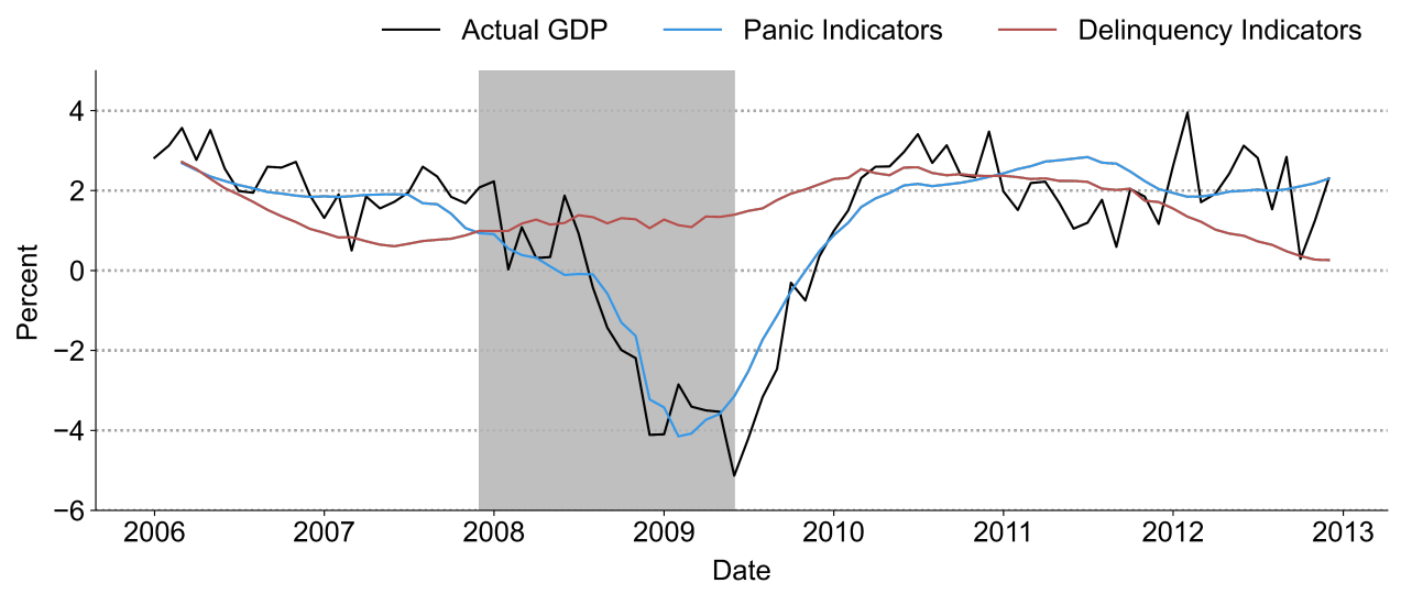
La Grande Récession
- La Grande Récession résulte de “ruptures de crédit”
- Une grande partie des intermédiaires étaient des shadow banks (banques d’investissement, sociétés de crédit hypothécaire, fonds monétaires, etc.) qui
- n’avaient pas accès aux prêts de la Federal Reserve comme les banques commerciales
- se finançaient à court terme
- étaient vulnérables aux paniques bancaires
- Bernanke (2018) montre que, pendant la crise, les mesures de panique financière (coûts de financement) prédisaient très bien les variables réelles
Cycles financiers
- Matteo Iacoviello
- travaille au Federal Reserve Board
- spécialisé en modélisation macro, notamment sur le marché immobilier
- Financial business cycles, Review of Economic Dynamics 2015
- modèle DSGE avec secteur financier et chocs financiers
- le modèle est estimé
- résultat : les récessions (cycles) sont déclenchées par des chocs de crédit
- Le modèle est plutôt simple du point de vue des microfondements
- … ce qui explique qu’il soit relativement mal publié
Résumé
Je considère une économie en temps discret.
L’économie comprend trois types d’agents : les ménages, les banquiers et les entrepreneurs. Chaque type a une masse unitaire.
Les ménages travaillent, consomment et achètent de l’immobilier, et placent des dépôts à une période auprès d’une banque. Le secteur des ménages est agrégativement épargnant net.
Les entrepreneurs accumulent de l’immobilier, embauchent des ménages et empruntent aux banques.
Entre ménages et entrepreneurs, les banquiers intermédient les fonds. La nature de l’activité bancaire implique que les banquiers sont emprunteurs vis-à-vis des ménages et prêteurs vis-à-vis du secteur dépendant du crédit, c’est-à-dire les entrepreneurs.
Les préférences sont construites de façon à ce que deux frictions coexistent et interagissent à l’équilibre : d’abord, les banquiers sont contraints en crédit dans la quantité qu’ils peuvent emprunter aux épargnants patients ; ensuite, les entrepreneurs sont contraints en crédit dans la quantité qu’ils peuvent emprunter aux banquiers.
Ménages
L’agent représentatif choisit le logement \(H_{H,t}\), la consommation \(C_{T,t}\) et le temps de travail \(N_{H,t}\) pour résoudre
\[\max E_t \sum_{t=0}^{\infty} \beta^t_H \left( \log C_{H,t} + j \log H_{H,t} + \tau \log(1-N_{H,t}) \right)\]
où \(\beta_{H,t}\) est le facteur d’actualisation et \(j,\tau\) deux paramètres de préférence.
. . .
sous la contrainte budgétaire :
\[C_{H,t} + D_t + q_t \left( H_{H,t}- H_{H,t-1} \right) = R_{H,t-1} D_{t-1} + W_{H,t} N_{H,t} + \epsilon_t\]
où :
- \(D_t\) : dépôts bancaires rémunérés au rendement brut \(R_{H,t}\)
- \(q_t\) : prix du logement
- \(W_t\) : salaire
- \(\epsilon_t\) : choc redistributif (proxy des défauts)
On obtient les conditions d’optimalité suivantes :
\[\frac{1}{C_{H,t}} = \beta_H E_t \left( \frac{1}{C_{H,t+1}} R_{H,t} \right)\] \[\frac{q_t}{C_{H,t}} = \frac{j}{H_{H,t}} + \beta_H E_t \left( \frac{q_{t+1}}{C_{H,t+1}} \right)\] \[\frac{W_{H,t}}{C_{H,t}} = \frac{\tau}{1-N_{H,t}}\]
Entrepreneurs
L’entrepreneur représentatif choisit la consommation \(C_{E,t}\), l’immobilier \(H_{H,t}\), la production \(Y_t\), le temps de travail \(N_{E,t}\), la dette \(L_{E,t}\): \[\max E_0 \sum_{t=0}^{\infty} \beta^t_E \log C_{E,t}\]
sous :
\[C_{E,t} + q_t \left( H_{E,t} - H_{E,t-1} \right) + R_{E,t} L_{E,t-1} + W_{H,t} N_{E,t} + a c_{EE,t} = Y_t + L_{E,t}\]
\[Y_t = H^{\nu}_{E,t-1} N^{1-\nu}_{E,t}\]
\[
L_{E,t} \leq m_H E_t \left( \frac{q_{t+1}}{R_{E,t+1}}H_{E,t} \right) - m_N W_{H,t} N_{E,t}
\tag{1}\]
\(L_{E,t}\) sont les prêts à l’entrepreneur, au rendement brut \(R_{E,t}\)
\(c_{EE,t}=\frac{\phi_{EE}}{2}\frac{\left(L_{E,t}-L_{E,t-1}\right)^ 2}{L_E}\) avec \(L_E\) l’état stationnaire de \(L_{E,t}\)
- capte le fait que les prêts évoluent lentement
Contrainte d’emprunt :
\[
L_{E,t} \leq m_H E_t \left( \frac{q_{t+1}}{R_{E,t+1}}H_{E,t} \right) - m_N W_{H,t} N_{H,t}
\tag{2}\]
- les entrepreneurs ne peuvent pas emprunter plus qu’une fraction \(m_H\) de la valeur anticipée de leur stock immobilier
- une fraction \(m_N\) de la masse salariale doit être payée d’avance
- les entrepreneurs ne peuvent pas emprunter pour la financer
Hypothèse : les entrepreneurs actualisent davantage le futur que les ménages et les banquiers
\[\beta_E < \frac{1}{\gamma_E \frac{1}{\beta_H} + (1-\gamma_E)\frac{1}{\beta_B}}\] avec \(\gamma_E\in[0,1]\)
Entrepreneurs : conditions d’optimalité
On obtient les conditions d’optimalité suivantes
\[\left( 1- \lambda_{E,t} - \frac{\partial ac_{LE,t}}{\partial L_{E,t}}\right) \frac{1}{c_{E,t}} = \beta_E E_t \left( R_{E,t+1} \frac{1}{c_{E,t+11}}\right)\]
\[\left(
q_t- \lambda_{E,t} m_H E_t \left( \frac{q_{t+1}}{R_{E,t+1}} \right)
\right)\frac{1}{c_{E,t}} = \beta_E E_t \left(
\left(q_{t+1} + \frac{\nu Y_{t+1}}{H_{E,t}}
\right)
\frac{1}{c_{E,t+1}}\right)
\]
\[\frac{(1-\nu)Y_t}{1+m_N \lambda_{E,t}}=W_{H,t} N_{H,t}\]
Commentaire : la contrainte de crédit introduit un écart entre le coût des facteurs et leur produit marginal.
- une distorsion comparable à une taxe
Banquiers
Le banquier représentatif maximise sa consommation privée \(C_{B,t}\)
\[\max E_0 \sum_{t=0}^{\infty} \beta^t_B \log C_{B,t}\]
\[C_{B,t} + R_{H,t-1} D_{t-1} + L_{E,t} + a c_{EB,t} = D_t + R_{E,t} L_{E,t-1} - \epsilon_t\]
où :
\(D_t\) : dépôts des ménages
\(L_{E,t}\) : prêts aux entrepreneurs
\(a c_{EB,t} = \frac{\phi_{EB}}{2} \frac{(L_{E,t-L_{E,t-1}})^2}{L_E}\) est un coût d’ajustement quadratique1
la capacité à transformer les dépôts en prêts est limitée par une contrainte d’emprunt2
\[D_t \leq \gamma_E \left( L_{E,t} - E_t \epsilon_{t+1} \right)\]
Banquiers (optimalité)
Notons :
- \(m_{B,t} = \beta_B \left( \frac{C_{B,t}}{C_{B,t+1}}\right)\) : le facteur d’actualisation stochastique du banquier
- \(\lambda_{B,t}\) : multiplicateur de la contrainte de fonds propres normalisé par l’utilité marginale de la consommation
Conditions d’optimalité :
\[1-\lambda_{B,t} = E_t \left( m_{B,t} R_{H,t} \right) \tag{3}\]
\[1-\gamma_{E} \lambda_{B,t} + \frac{\partial ac_{EB,t}}{\partial L_{E,t}} = E_t \left( m_{B,t} R_{E,t+1} \right) \tag{4}\]
Ces deux équations expliquent l’écart entre le taux de dépôt et le taux de prêt (la prime d’intermédiation)
Banquiers (optimalité)
\[1-\lambda_{B,t} = E_t \left( m_{B,t} R_{H,t} \right)\]
\[1-\gamma_{E} \lambda_{B,t} + \frac{\partial ac_{EB,t}}{\partial L_{E,t}} = E_t \left( m_{B,t} R_{E,t+1} \right)\]
Interprétation :
- le banquier peut consommer davantage en empruntant aux ménages pour financer sa consommation
- cela resserre sa contrainte de crédit
- cela réduit la valeur d’un dépôt supplémentaire de \(\lambda_{B,t}\)
- le banquier peut consommer davantage en réduisant les prêts
- cela resserre aussi sa contrainte de crédit (baisse des fonds propres)
- l’effet est plus fort si l’exigence de collatéraux est plus élevée
Equilibre des marches
Conditions d’equilibre sur logement :
\[H_{E,t} + H_{H,t} = 1\]
Conditions d’equilibre sur les marches du travail :
\[N_{H,t} = N_{E,t}\]
Conditions d’equilibre sur le marché des biens:
\[Y_t = C_{H,t} + C_{E,t} + C_{E,t} + a c_{EE,t} + a c_{EB,t}\]
Proprietes de l’etat stationnaire
Pour les ménages :
\[R_H=\frac{1}{\beta_H}\]
Pour les banquiers :
Equation 3 et Equation 4 impliquent que tant que \(\beta_B<\beta_H\), les banquiers sont contraints en crédit
Avec \(\gamma_{E}\) inférieur à 1, il existe un spread entre le rendement des prêts et celui des dépôts :
\[\lambda_B = 1-\beta_B R_H = 1-\frac{\beta_B}{\beta_H}>0\]
\[R_E = \frac{1}{\beta_B} - \gamma_E \left( \frac{1}{\beta_B} - \frac{1}{\beta_H} \right)>R_H\]
Pour les entrepreneurs
Les entrepreneurs sont contraints si \(\beta_E R_E<1\). Ce qui est équivalent à \[\frac{1}{\beta_E}=\gamma_E \frac{1}{\beta_H} + (1-\gamma_E) \frac{1}{\beta_B}\]
Effet :
- les contraintes de crédit des banquiers et des entrepreneurs créent un écart et réduisent la production de long terme
Hypothèse technique : à l’état stationnaire, les contraintes sont saturantes. Iacoviello suppose qu’elles le restent dans un voisinage de l’état stationnaire.
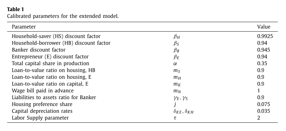
Calibration
Période de temps : 1 trimestre
Facteurs d’actualisation :
- ménages : \(\beta_H=0.9925\)
- banquiers : \(\beta_B=0.945\)
- entrepreneurs : \(\beta_E=0.94\)
Choix des paramètres de levier de sorte que \(R_H=3\%\) et \(R_E=5\%\).
Coûts d’ajustement : \(\phi_{EE}=\phi_{EB}=0.25\)
Poids du loisir dans l’utilité : \(\tau=2\) (temps de travail actif = 1/2 et élasticité de Frisch1 proche de 1).
Part du logement dans la production : \(\nu=0.05\)
Paramètre de préférence pour le logement \(j=0.075\) : ratio richesse immobilière / production = 3,1 (0,8 commercial, 2,3 résidentiel)
Levier :
- \(m_N=1\) : tout le travail est payé d’avance
- \(m_H=0.9\) : loan-to-value (LTV) des entrepreneurs
- \(\gamma_E=0.9\) : levier bancaire (proche des ratios historiques de capital sur actifs)
Dynamique
Dynamique du spread d’intermédiation
\[E_t \left( R_{E,t+1} \right) - R_{H,t} = \frac{\lambda_{B,t}}{m_{B,t}}(1-\gamma_E)\]
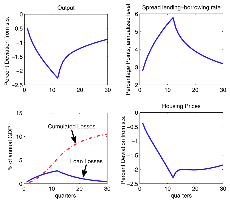
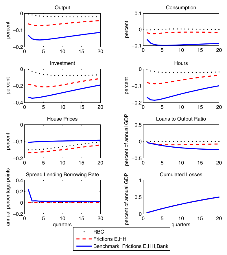
Première simulation
Le choc \(\epsilon_t\) est calibré sur les pertes historiques sur prêts (montants de dépréciation de dette)
On a \[\epsilon_t = 0.9 \epsilon_{t-1} + \iota_t\]
La déviation exogène est la suivante :
- hausse de 0,38% du PIB chaque trimestre pendant 12 trimestres
- les pertes du système financier passent de 0 à 2,8% après 2 ans
- retour progressif vers zéro
Première simulation
![]()
Modèle étendu
Le modèle complet contient :
- deux types de ménages :
- habitudes de consommation + chocs de préférence \[\max E_t\sum_t \beta^t \log(C_t -\eta C_{H,t-1}) + j A_{j,t} \log(H_{H,t}) + \tau \log(1-N_{H,t})\]
- chocs sur toutes les capacités d’emprunt
- chocs d’efficacité de l’investissement + chocs de PTF
Modèle estimé par une approche bayésienne de 1985 à 2010
- 8 chocs au total
- 8 variables observables
Calibration
![]()
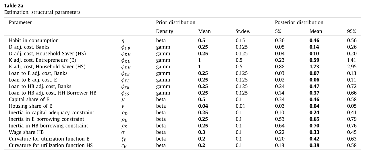
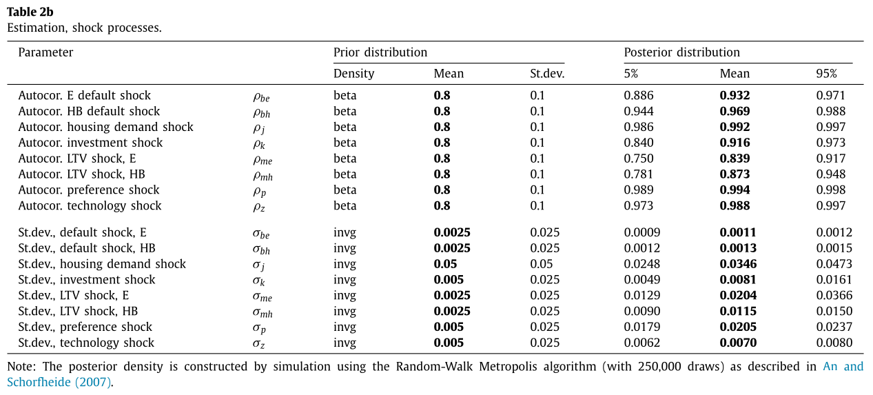
Résultats d’estimation
![]()
Résultats d’estimation
![]()
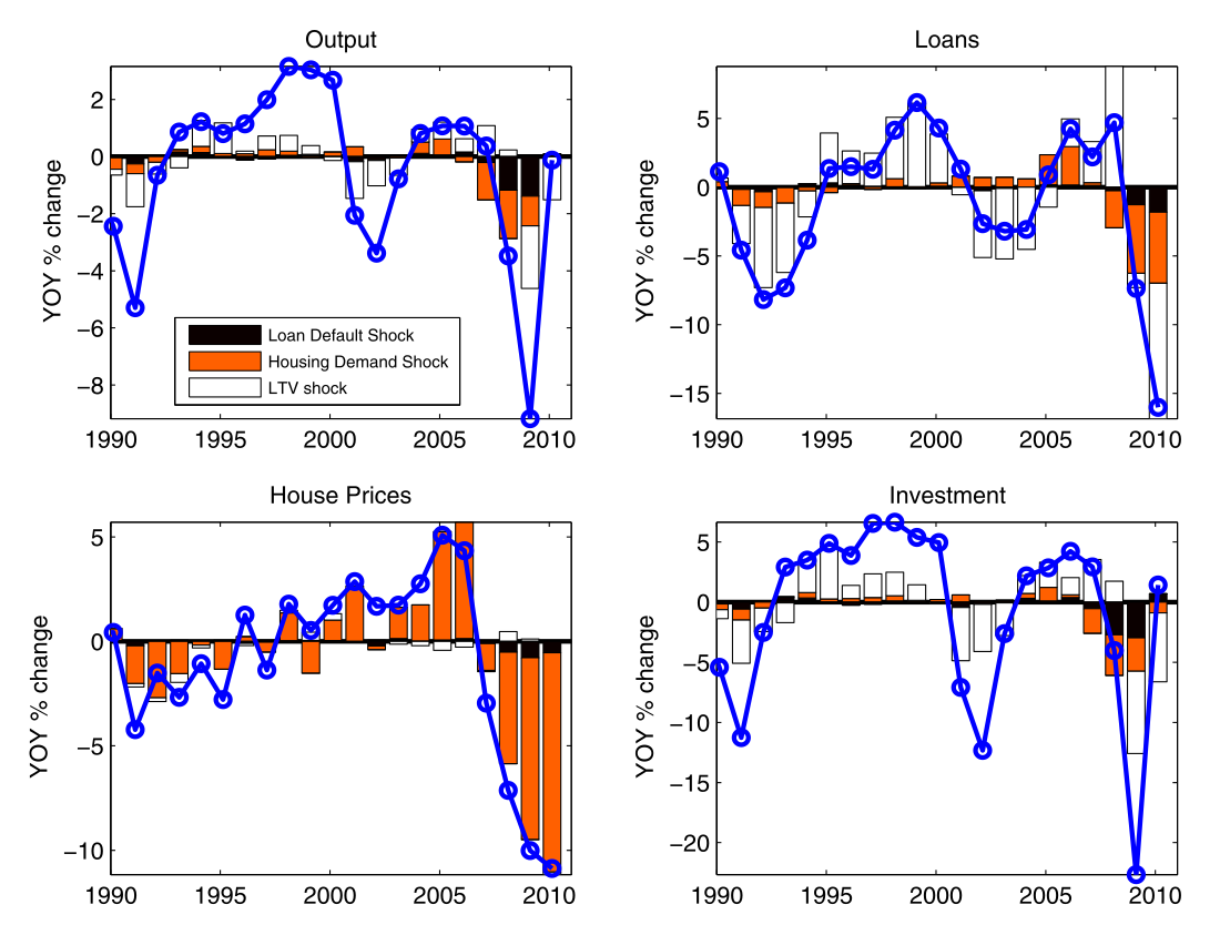
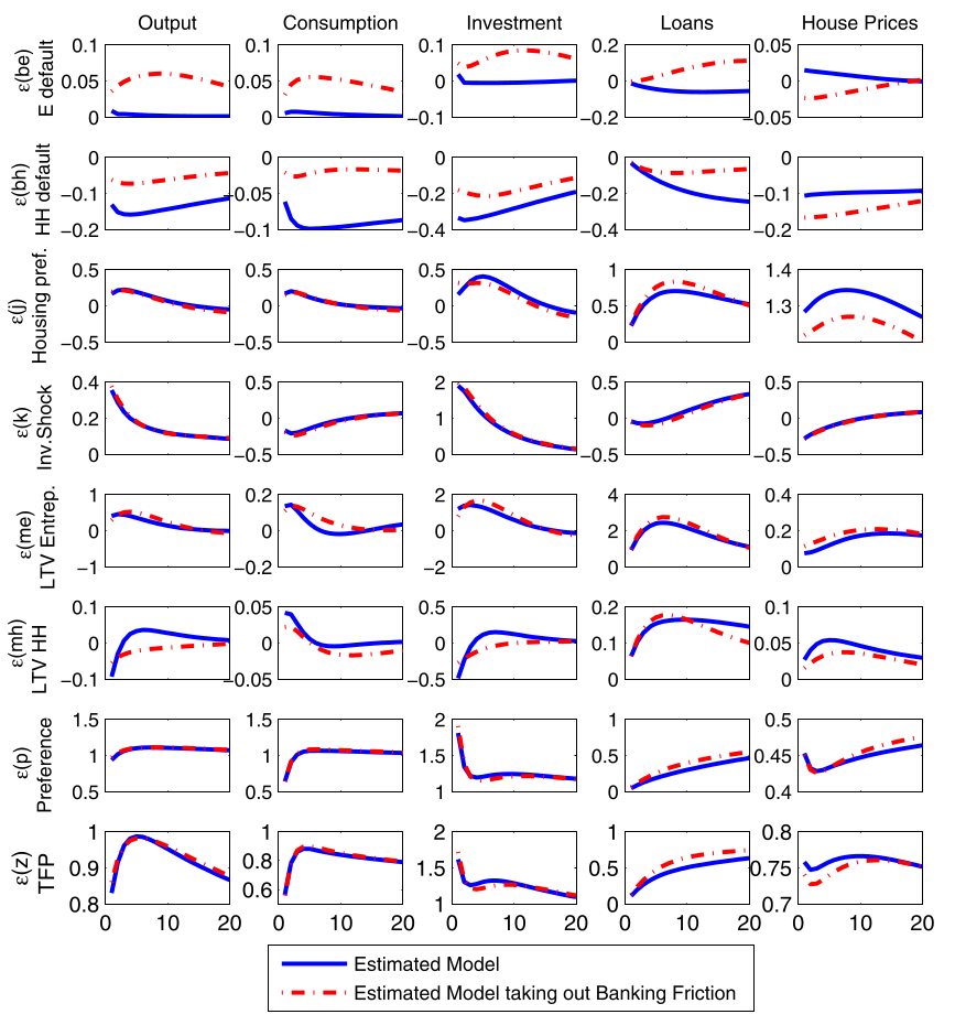
Identification
![]()
Un modèle estimé peut être utilisé pour identifier les chocs.
- l’essentiel des variations des prix immobiliers et des volumes de crédit peut être attribué aux chocs financiers
- une part importante des fluctuations de la production et de l’investissement aussi
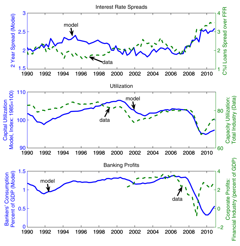
Pouvoir prédictif du modèle
![]()
Pouvoir prédictif du modèle
Le modèle prédit aussi d’autres moments qui n’étaient pas ciblés :
- spreads de taux d’intérêt
- taux d’utilisation des capacités
- profits des entreprises \(\approx\) consommation des banquiers
Conclusion
Le modèle FBC montre que les chocs financiers ont probablement été un moteur de la crise financière (🤔)
Mais il manque :
- un modèle microfondé et réaliste des banques
- un rôle pour la banque centrale et la création monétaire
- en particulier la création monétaire par les banques…
- un environnement macroéconomique plus réaliste
- en particulier, le capital