Optimization
Macroeconomics: Numerical Methods
2025-04-04
Introduction
Introduction
Optimization is everywhere in economics:
- to model agent’s behaviour: what would a rational agent do?
- consumer maximizes utility from consumption
- firm maximizes profit
- an economist tries to solve a model:
- find prices that clear the market
Two kinds of optimization problem:
root finding: \(\text{find $x$ in $X$ such that $f(x)=0$}\)
minimization/maximization \(\min_{x\in X} f(x)\) or \(\max_{x\in X} f(x)\)
often a minimization problem can be reformulated as a root-finding problem
\[x_0 = {argmin}_{x\in X} f(x) \overbrace{\iff}^{??} f^{\prime} (x_0) = 0\]
Plan
- general consideration about optimization problems
- one-dimensional root-finding
- one-dimensional optimization
- local root-finding
- local optimization
- constrained optimization
- constrained root-finding
General considerationsre
Optimization tasks come in many flavours
- continuous versus discrete optimization
- constrained and unconstrained optimization
- global and local
- stochastic and deterministic optimization
- convexity
Continuous versus discrete optimization
- Choice is picked from a given set (\(x\in X\)) which can be:
- continuous: choose amount of debt \(b_t \in [0,\overline{b}]\), of capital \(k_t \in R^{+}\)
- discrete: choose whether to repay or default \(\delta\in{0,1}\), how many machines to buy (\(\in N\)), at which age to retire…
- a combination of both: mixed integer programming
Continuous versus discrete optimization (2)
- Discrete optimization requires a lot of combinatorial thinking
- We don’t cover it today.
- …if needed, we just test all choices until we find the best one
- Sometimes a discrete choice can be approximated by a mixed strategy (i.e. a random strategy).
- Instead of \(\delta\in{0,1}\) we choose \(x\) in \(prob(\delta=1)=\sigma(x)\)
- with \(\sigma(x)=\frac{2}{1+\exp(-x)}\)
Constrained and Unconstrained optimization
- Unconstrained optimization: \(x\in R\)
- Constrained optimization: \(x\in X\)
- budget set: \(p_1 c_1 + p_2 c_2 \leq I\)
- positivity of consumption: \(c \geq 0\).
- In good cases, the optimization set is convex…
- pretty much always in this course
Stochastic vs Determinstic
- Common case, especially in machine learning \[f(x) = E_{\epsilon}[ \xi (\epsilon, x)]\]
- One wants to maximize (resp solve) w.r.t. \(x\) but it is costly to compute expectation precisely using Monte-Carlo draws (there are other methods).
- A stochastic optimization method allows to use noisy estimates of the expectation, and will still converge in expectation.
- For now we focus on deterministic methods. Maybe later…
Local vs global Algorithms
In principle, there can be many roots (resp maxima) within the optimization set.
Algorithms that find them all are called “global”. For instance:
- grid search
- simulated annealing
We will deal only with local algorithms, and consider local convergence properties.
- ->then it might work or not
- to perform global optimization just restart from different points.
Math vs practice
The full mathematical treatment will typically assume that \(f\) is smooth (\(\mathcal{C}_1\) or \(\mathcal{C}_2\) depending on the algorithm).
In practice we often don’t know about these properties
- we still try and check thqt we have a local optimal
So: fingers crossed
Math vs practice
Here is the surface representing the objective that a deep neural network training algorithm tries to minimize.
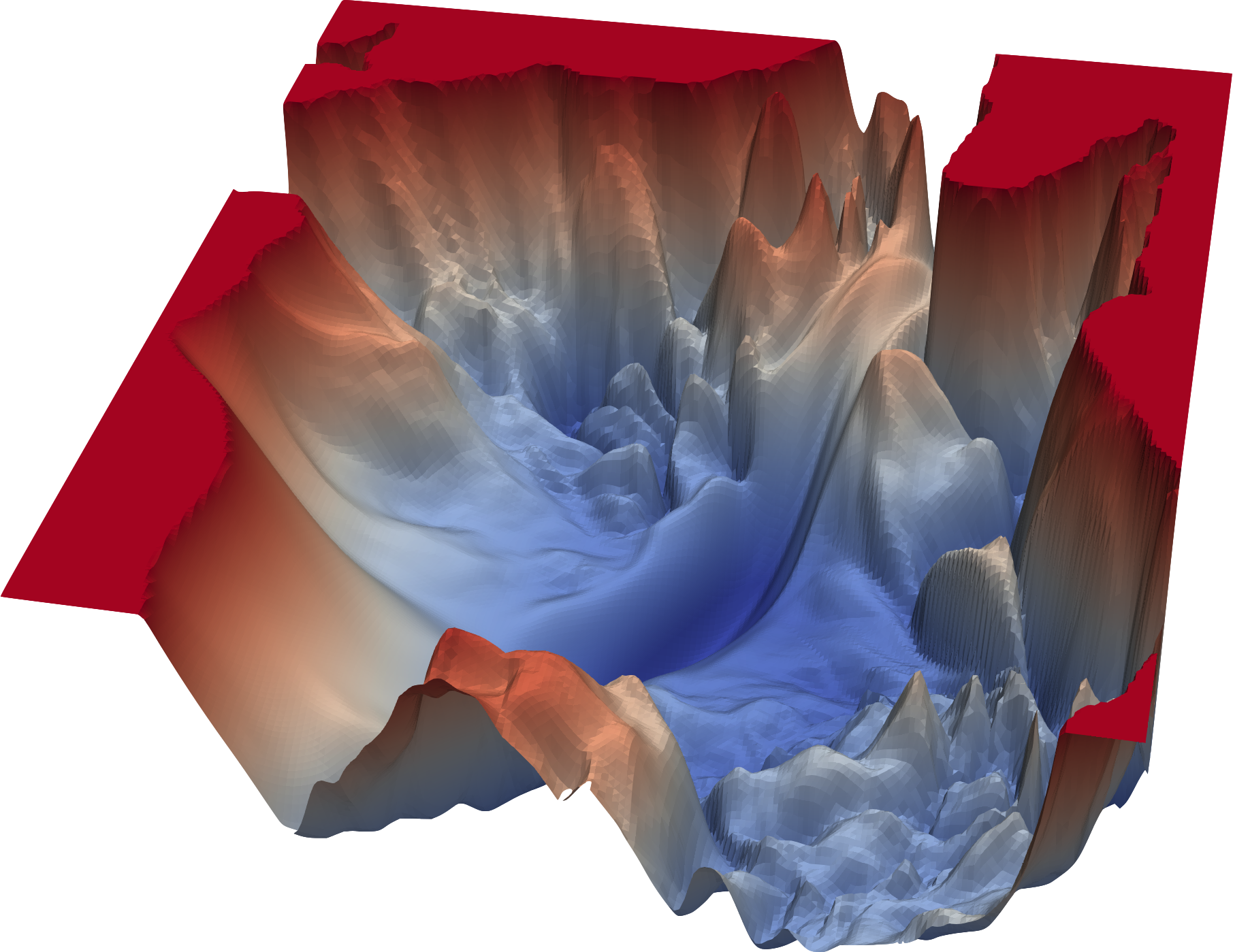
And yet, neural networks do great things!
What do you need to know?
- be able to handcode simple algos (Newton, Gradient Descent)
- understand the general principle of the various algorithms to compare them in terms of
- robustness
- efficiency
- accuracy
- then you can just switch the various options, when you use a library…
One-dimensional root-finding
Bisection
- Find \(x \in [a,b]\) such that \(f(x) = 0\). Assume \(f(a)f(b) <0\).
- Algorithm
- Start with \(a_n, b_n\). Set \(c_n=(a_n+b_n)/2\)
- Compute \(f(c_n)\)
- if \(f(c_n)f(a_n)<0\) then set \((a_{n+1},b_{n+1})=(a_n,c_n)\)
- else set \((a_{n+1},b_{n+1})=(c_n,b_n)\)
- If \(|f(c_n)|<\epsilon\) and/or \(\frac{b-a}{2^n}<\delta\) stop. Otherwise go back to 1.
Bisection (2)
- No need for initial guess: globally convergent algorithm
- not a global algorithm…
- … in the sense that it doesn’t find all solutions
- \(\delta\) is a guaranteed accuracy on \(x\)
- \(\epsilon\) is a measure of how good the solution is
- think about your tradeoff: (\(\delta\) or \(\epsilon\) ?)
Newton algorithm
- Find \(x\) such that \(f(x) = 0\). Use \(x_0\) as initial guess.
- \(f\) must be \(\mathcal{C_1}\) and we assume we can compute its derivative \(f^{\prime}\)
- General idea:
- observe that the zero \(x^{\star}\) must satisfy \[f(x^{\star})=0=f(x_0)+f^{\prime}(x_0)(x^{\star}-x_0) + o(x-x_0)\]
- Hence a good approximation should be \[x^{\star}\approx = x_0- f(x_0)/f^{\prime}(x_0)\]
- Check it is good. otherwise, replace \(x_0\) by \(x^{\star}\)
Newton algorithm (2)
- Algorithm:
- start with \(x_n\)
- compute \(x_{n+1} = x_n- \frac{f(x_n)}{f^{\prime}(x_n)}=f^{\text{newton}}(x_n)\)
- stop if \(|x_{n+1}-x_n|<\eta\) or \(|f(x_n)| < \epsilon\)
- Convergence: quadratic
Quasi-Newton
- What if we can’t compute \(f^{\prime}\) or it is expensive to do so?
- Idea: try to approximate \(f^{\prime}(x_n)\) from the last iterates
- Secant method: \[f^{\prime}(x_n)\approx \frac{f(x_n)-f(x_{n-1})}{x_n-x_{n-1}}\] \[x_{n+1} = x_n- f(x_n)\frac{x_n-x_{n-1}}{f(x_n)-f(x_{n-1})}\]
- requires two initial guesses: \(x_1\) and \(x_0\)
- superlinear convergence: \(\lim \frac{x_t-x^{\star}}{x_{t-1}-x^{\star}}\rightarrow 0\)
Limits of Newton’s method
- How could Newton method fail?
- bad guess
- -> start with a better guess
- overshoot
- -> dampen the update (problem: much slower)
- -> backtrack
- stationary point
- -> if root of multiplicity \(m\) try \(x_{n+1} = x_n- m \frac{f(x_n)}{f^{\prime}(x_n)}\)
- bad guess
(some graphs of failed Newton convergence)
Backtracking
- Simple idea:
- at stage \(n\) given \(f(x_n)\) compute Newton step \(\Delta_n=-\frac{f(x_n)}{f^{\prime}(x_n)}\)
- find the smallest \(k\) such that \(|f(x_n-\Delta/2^k)|<|f(x_n)|\)
- set \(x_{n+1}=x_n-\Delta/2^k\)
One dimensional minimization
Golden section search
Minimize \(f(x)\) for \(x \in [a,b]\)
Choose \(\Phi \in [0,0.5]\)
Algorithm:
- start with \(a_n < b_n\) (initially equal to \(a\) and \(b\))
- define \(c_n = a_n+\Phi(b_n-a_n)\) and \(d_n = a_n+(1-\Phi)(b_n-a_n)\)
- if \(f(c_n)<f(d_n)\) set \(a_{n+1},b_{n+1}=a_n, d_n\)
- else set \(a_{n+1}, b_{n+1}= c_n, b_n\)
Golden section search (2)
- This is guaranteed to converge to a local minimum
- In each step, the size of the interval is reduced by a factor \(\Phi\)
- By choosing \(\Phi=\frac{\sqrt{5}-1}{2}\) one can save one evaluation by iteration.
- you can check that either \(c_{n+1} = d_n\) or \(d_{n+1} = c_n\)
- Remark that bisection is not enough
Gradient Descent
- Minimize \(f(x)\) for \(x \in R\) given initial guess \(x_0\)
- Algorithm:
- start with \(x_n\)
- compute \(x_{n+1} = x_n (1-\lambda)- \lambda f^{\prime}(x_n)\)
- stop if \(|x_{n+1}-x_n|<\eta\) or \(|f^{\prime}(x_n)| < \epsilon\)
Gradient Descent (2)
- Uses local information
- one needs to compute the gradient
- note that gradient at \(x_n\) does not provide a better guess for the minimum than \(x_n\) itself
- learning speed is crucial
- Convergence speed: linear
- rate depend on the learning speed
- optimal learning speed? the fastest for which there is convergence
Newton-Raphson method
- Minimize \(f(x)\) for \(x \in R\) given initial guess \(x_0\)
- Build a local model of \(f\) around \(x_0\) \[f(x) = f(x_0) + f^{\prime}(x_0)(x-x_0) + f^{\prime\prime}(x_0)\frac{(x-x_0)^2}{2} + o(x-x_0)^2\]
- According to this model, \[ f(x{\star}) = min_x f(x)\iff \frac{d}{d x} \left[ f(x_0) + f^{\prime}(x_0)(x-x_0) + f^{\prime\prime}(x_0)\frac{(x-x_0)^2}{2} \right] = 0\] which yields: \(x^{\star} = x_0 - \frac{f^{\prime}(x_0)}{f^{\prime\prime}(x_0)}\)
- this is Newton applied to \(f^{\prime}(x)=0\)
Newton-Raphson Algorithm (2)
- Algorithm:
- start with \(x_n\)
- compute \(x_{n+1} = x_n-\frac{f^{\prime}(x_0)}{f^{\prime\prime}(x_0)}\)
- stop if \(|x_{n+1}-x_n|<\eta\) or \(|f^{\prime}(x_n)| < \epsilon\)
- Convergence: quadratic
Unconstrained Multidimensional Optimization
Unconstrained problems
Minimize \(f(x)\) for \(x \in R^n\) given initial guess \(x_0 \in R^n\)
Many intuitions from the 1d case, still apply
- replace derivatives by gradient, jacobian and hessian
- recall that matrix multiplication is not commutative
Some specific problems:
- update speed can be specific to each dimension
- saddle-point issues (for minimization)
Quick terminology
Function \(f: R^p \rightarrow R^q\)
Jacobian: \(J(x)\) or \(f^{\prime}\_x(x)\), \(p\times q\) matrix such that: \[J(x)\_{ij} = \frac{\partial f(x)\_i}{\partial x_j}\]
Gradient: \(\nabla f(x) = J(x)\), gradient when \(q=1\)
Hessian: denoted by \(H(x)\) or \(f^{\prime\prime}\_{xx}(x)\) when \(q=1\): \[H(x)\_{jk} = \frac{\partial f(x)}{\partial x_j\partial x_k}\]
In the following explanations, \(|x|\) denotes the supremum norm, but most of the following explanations also work with other norms.
Unconstrained Multidimensional Root-Finding
Multidimensional Newton-Raphson
- Algorithm:
- start with \(x_n\)
- compute \(x_{n+1} = x_n- J(x_{n})^{-1}f(x_n)=f^{\text{newton}}(x_n)\)
- stop if \(|x_{n+1}-x_n|<\eta\) or \(|f(x_n)| < \epsilon\)
- Convergence: quadratic
Multidimensional Newton root-finding (2)
- what matters is the computation of the step \(\Delta_n = {\color{\red}{J(x_{n})^{-1}}} f(x_n)\)
- don’t compute \(J(x_n)^{-1}\)
- it takes less operations to compute \(X\) in \(AX=Y\) than \(A^{-1}\) then \(A^{-1}Y\)
- in Julia:
X = A \ Y
- strategies to improve convergence:
- dampening: \(x_n = (1-\lambda)x_{n-1} - \lambda \Delta_n\)
- backtracking: choose \(k\) such that \(|f(x_n-2^{-k}\Delta_n)|\)<\(|f(x_{n-1})|\)
- linesearch: choose \(\lambda\in[0,1]\) so that \(|f(x_n-\lambda\Delta_n)|\) is minimal
Unconstrained Multidimensional Minimization
Multidimensional Gradient Descent
- Minimize \(f(x) \in R\) for \(x \in R^n\) given \(x_0 \in R^n\)
- Algorithm
- start with \(x_n\) \[x_{n+1} = (1-\lambda) x_n - \lambda \nabla f(x_n)\]
- stop if \(|x_{n+1}-x_n|<\eta\) or \(|f(x_n)| < \epsilon\)
- Comments:
- lots of variants
- automatic differentiation software makes gradient easy to compute
- convergence is typically linear
Gradient descent variants
Multidimensional Newton Minimization
- Algorithm:
- start with \(x_n\)
- compute \(x_{n+1} = x_n-{\color{\red}{H(x_{n})^{-1}}}\color{\green}{ J(x_n)'}\)
- stop if \(|x_{n+1}-x_n|<\eta\) or \(|f(x_n)| < \epsilon\)
- Convergence: quadratic
- Problem:
- \(H(x_{n})\) hard to compute efficiently
- rather unstable
Quasi-Newton method for multidimensional minimization
- Recall the secant method:
- \(f(x_{n-1})\) and \(f(x_{n-2})\) are used to approximate \(f^{\prime}(x_{n-2})\).
- Intuitively, \(n\) iterates would be needed to approximate a hessian of size \(n\)….
- Broyden method: takes \(2 n\) steps to solve a linear problem of size \(n\)
- uses past information incrementally
Quasi-Newton method for multidimensional minimization
- Consider the approximation: \[f(x_n)-f(x_{n-1}) \approx J(x_n) (x_n - x_{n-1})\]
- \(J(x_n)\) is unknown and cannot be determined directly as in the secant method.
- idea: \(J(x_n)\) as close as possible to \(J(x_{n-1})\) while solving the secant equation
- formula: \[J_n = J_{n-1} + \frac{(f(x_n)-f(x_{n-1})) - J_{n-1}(x_n-x_{n-1})}{||x_n-x_{n-1}||^2}(x_n-x_{n-1})^{\prime}\]
Gauss-Newton Minimization
- Restrict to least-square minimization: $min_x _i f(x)_i^2 R $
- Then up to first order, \(H(x_n)\approx J(x_n)^{\prime}J(x_n)\)
- Use the step: \(({J(x_n)^{\prime}J(x_n)})^{-1}\color{\green}{ J(x_n)}\)
- Convergence:
- can be quadratic at best
- linear in general
Levenberg-Marquardt
Least-square minimization: $min_x _i f(x)_i^2 R $
replace \({J(x_n)^{\prime}J(x_n)}^{-1}\) by \({J(x_n)^{\prime}J(x_n)}^{-1} +\mu I\)
- adjust \(\lambda\) depending on progress
uses only gradient information like Gauss-Newton
equivalent to Gauss-Newton close to the solution (\(\mu\) small)
equivalent to Gradient far from solution (\(\mu\) high)
Constrained optimization and complementarity conditions
Consumption optimization
Consider the optimization problem: \[\max U(x_1, x_2)\]
under the constraint \(p_1 x_1 + p_2 x_2 \leq B\)
where \(U(.)\), \(p_1\), \(p_2\) and \(B\) are given.
How do you find a solution by hand?
Consumption optimization (1)
- Compute by hand
- Easy:
- since the budget constraint must be binding, get rid of it by stating \(x_2 = B - p_1 x_1\)
- then maximize in \(x_1\), \(U(x_1, B - p_1 x_1)\) using the first order conditions.
- It works but:
- breaks symmetry between the two goods
- what if there are other constraints: \(x_1\geq \underline{x}\)?
- what if constraints are not binding?
- is there a better way to solve this problem?
Consumption optimization (2)
- Another method, which keeps the symmetry. Constraint is binding, trying to minimize along the budget line yields an implicit relation between \(d x_1\) and \(d x_2\) \[p_1 d {x_1} + p_2 d {x_2} = 0\]
- At the optimal: \(U^{\prime}\_{x_1}(x_1, x_2)d {x_1} + U^{\prime}\_{x_2}(x_1, x_2)d {x_2} = 0\)
- Eliminate \(d {x_1}\) and \(d {x_2}\) to get one condition which characterizes optimal choices for all possible budgets. Combine with the budget constraint to get a second condition.
Penalty function
- Take a penalty function \(p(x)\) such that \(p(x)=K>0\) if \(x>0\) and \(p(x)=0\) if \(x \leq 0\). Maximize: \(V(x_1, x_2) = U(x_1, x_2) - p( p_1 x_1 + p_2 x_2 - B)\)
- Clearly, \(\min U \iff \min V\)
- Problem: \(\nabla V\) is always equal to \(\nabla U\).
- Solution: use a smooth solution function like \(p(x) = x^2\)
- Problem: distorts optimization
- Solution: adjust weight of barrier and minimize \(U(x_1, x_2) - \kappa p(x)\)
- Possible but hard to choose the weights/constraints.
Penalty function
- Another idea: is there a canonical way to choose \(\lambda\) such that at the minimum it is equivalent to minimize the original problem under constraint or to minimize \[V(x_1, x_2) = U(x_1, x_2) - \lambda (p_1 x_1 + p_2 x_2 - B)\]
- Clearly, when the constraint is not binding we must have \(\lambda=0\). What should be the value of \(\lambda\) when the constraint is binding ?
Karush-Kuhn-Tucker conditions
- If \((x^{\star},y^{\star})\) is optimal there exists \(\lambda\) such that:
- \((x^{\star},y^{\star})\) maximizes lagrangian \(\mathcal{L} = U(x_1, x_2) + \lambda (B- p_1 x_1 - p_2 x_2)\)
- \(\lambda \geq 0\)
- \(B- p_1 x_1 - p_2 x_2 \geq 0\)
- \(\lambda (B - p_1 x_1 - p_2 x_2 ) = 0\)
- The three latest conditions are called “complementarity” or “slackness” conditions
- they are equivalent to \(\min(\lambda, B - p_1 x_1 - p_2 x_2)=0\)
- we denote \(\lambda \geq 0 \perp B- p_1 x_1 + p_2 x_2 \geq 0\)
- \(\lambda\) can be interpreted as the welfare gain of relaxing the constraint.
Karush-Kuhn-Tucker conditions
- We can get first order conditions that factor in the constraints:
- \(U^{\prime}_x - \lambda p_1 = 0\)
- \(U^{\prime}_y - \lambda p_2 = 0\)
- \(\lambda \geq 0 \perp B-p_1 x_1 -p_2 x_2 \geq 0\)
- It is now a nonlinear system of equations with complementarities (NCP)
- there are specific solution methods to deal with it
Solution strategies for NCP problems
General formulation for vector-valued functions \[f(x)\geq 0 \perp g(x)\geq 0\] means \[\forall i, f_i(x)\geq 0 \perp g_i(x)\geq 0\]
- NCP do not necessarily arise from a single optimization problem
There are robust (commercial) solvers for NCP problems (PATH, Knitro) for that
How do we solve it numerically?
- assume constraint is binding then non-binding then check which one is good
- OK if not too many constraints
- reformulate it as a smooth problem
- approximate the system by a series of linear complementarities problems (LCP)
- assume constraint is binding then non-binding then check which one is good
Smooth method
- Consider the Fisher-Burmeister function \[\phi(a,b) = a+b-\sqrt{a^2+b^2}\]
- It is infinitely differentiable, except at \((0,0)\)
- Show that \(\phi(a,b) = 0 \iff \min(a,b)=0 \iff a\geq 0 \perp b \geq 0\)
- After substitution in the original system one can use regular non-linear solver
- fun fact: the formulation with a \(\min\) is nonsmooth but also works quite often
Practicalities
Optimization libraries
- Robust optimization code is contained in the following libraries:
- Roots.jl: one-dimensional root finding
- NLSolve.jl: multidimensional root finding (+complementarities)
- Optim.jl: minimization
- The two latter libraries have a somewhat peculiar API, but it’s worth absorbing it.
- in particular they provide non-allocating algorithms for functions that modify arguments in place
- they are compatible with automatic differentiation
julia> f(x) = [x[1] - x[2] - 1, x[1] + x[2]]
f (generic function with 1 method)

julia> NLsolve.nlsolve(f, [0., 0.0])
Results of Nonlinear Solver Algorithm
 * Algorithm: Trust-region with dogleg and autoscaling
 * Starting Point: [0.0, 0.0]
 * Zero: [0.5000000000009869, -0.5000000000009869]
 * Inf-norm of residuals: 0.000000
 * Iterations: 1
 * Convergence: true
   * |x - x'| < 0.0e+00: false
   * |f(x)| < 1.0e-08: true
 * Function Calls (f): 2
* Jacobian Calls (df/dx): 2![]()